1. Introduction

This text is a significantly changed extension of the work firstly presented as a conference paper [1].

The global world has been already transferring into the information society for several recent decades. It is quite acceptable to consider a Geographic Information System – GIS as one of the core tools of such transfer together with the relevant technologies of remote sensing, including LiDAR (Light Detection and Ranging) technique. It has been remarkable for few recent decades that exactly this period also has been featured by the continuing urbanization process, that still takes place nowadays in many developing countries. Numerous facts and phenomena indicate, that we may face the largest urban growth wave within the whole human history, which also concurs with prompt development of information technologies, remote sensing, computer sciences, geoinformatics, and GIS-platforms / modules. All listed entities could and should be involved in resolving of those drastic problems arisen within the urbanized areas, for example, by considering these territories as the hierarchical urban geosystems and making the corresponding decision support recommendations [2, 3]. Thus, even several highly challenging issues relevant to the Smart City development can be met in this way [4]. Moreover, the rapid growth of both remote sensing technique and GIS-technological involvement in surveying environmental consequences of the urbanization process has been clear evident over the past few decades [5], while quite a few both approaches, and methods, as well as user interfaces have been developed [6-15].

Urban features can be accepted as the core constituents of any virtual presentation for each digitally simulated city. A 3D City Model is the key formalized entity of the mentioned city content, and it enables effective and accurate 3D modeling of the urbanized environment with respects to housing sets and infrastructures [16-23]. Within the urban studies perspectives it can be possible to accept a 3D object / feature model as a work-flow key issue of the GIS output completed from the urban remote sensing input. This assumption may be even more evident, while the discrete objects are considered as those modeled results, which are intended for a customized solution within the framework of one only, or several urban applications. In this meaning 3D modeling appears to become a key component within the common geoinformation paradigm [24]. It is considered be possible to accept a 3D city model of urban area as that entity, which corresponding environmental analog is placed within 3D urban environment described by routine urban features and structures with buildings as the dominant objects among them.

Exactly for a couple of latest decades LiDAR (Lidar) data collecting processing technique has become an alternative (to areal imageries) data source for generating a 3D representation of natural landscapes and housing environments as well as the overall human-environment intercourse [25, 26]. Being able to collect directly the accurate 3D point clouds of various density over urban territories, the LiDAR technique proposes an effective and beneficial data source in this meaning. By the way, this is illustrated further in this text.

There are Airborne (ALS), Terrestrial (Mobile – MLS), and UAV-LS (Unmanned Aerial Vehicle Laser Scanning) LiDAR techniques within the common remote sensing technology, that measures distances on the base of the time intervals between the laser signal transmitting / receiving. All ALS / MLS /UAV-LS mapping are surveying and mapping tools based on hardware platforms and software solutions [27-30]. The ALS lidar normally completes low-average density measurements of the underlying topographic surface, that result in the georeferenced, but unstructured set of points – lidar Point Clouds, while the MLS technique usually captures the walls – with a high resolution of façade details for buildings of different sizes. The UAV-LS lidar accomplishes high density measurements and can provide surveys that may be considered as hybrid ones, since it combines those output data, which can be provided by both ALS, and MLS Lidars.

The automated feature extraction (AFE) methods are the derivatives of ALS / MLS / UAV-LS Lidar remote technique. AFE-procedures produce 3D city models mentioned above, that are positioned in three dimensions just because of the AFE-method implementation. Since a common three-dimensional urban model may be a subject of more, than one hundred applications in various industrial domains [24], the AFE-methodology itself can be hardly overvalued. Municipal management, urban emergency services, noise and other hazard mapping, visibility analysis city infrastructure inventory, population and energy demand estimation with building models are those key urban applications, in which 3D models obtained from LiDAR data through AFE procedures are in an evident growing marketing demand according to the obvious reasons. To meet this demand requirements an AFE-model should be of high accuracy [31], what in some cases implies a hybrid data source. The latter means either a “LiDAR + areal image” hybrid [32], or additional involvement of MLS / UAV-LS data processing procedures for detailed extractions of building façades [33].

The main research purpose of this text is to outline with the phased methodological flowchart our conceptual multifunctional approach to the fully automated extraction of urban features, and present the original contribution to relevant algorithmic solutions within the modeling pipeline, as well as represent the web- and cloud-based software elaborated for these intentions.

2. Previous Works Done due to Building Detection, Extraction, and 3D Reconstruction from LiDAR Data

Fully Automated Feature Extraction, building Point Cloud segmentation, rooftop modeling, and 3D reconstruction of buildings, all have been among the main topics of thematic discussions in the remote sensing community through the relevant papers and on forums of various scales especially for the latest decade [26, 32, 34-42].

Now, AFE is still a vitally crucial part of what is being done and what researchers and other professionals are attempting to do better within the LiDAR surveying / processing domain. How has it further been progressed with its technique recently? We may consider as a key issue for efficient AFE-results a provision of a bridge between MLS / UAV-LS lidars, from one side, and ALS lidar, from another, one and vice-versa. Without any further explanations just in this paper section, we may only express a somewhat trivial idea, according to which the composite models of urban features extracted may be considered as the most effective ones [43].

2.1.  Overall AFE issues

Because of ALS / MLS / UAV-LS joint surveying methods the automated feature extraction as a generating procedure for 3D urban models has become an evident alternative to the urban photogrammetry. It is a well-known fact, that besides various direct processing of aerial images, the Urban Remote Sensing (URS) (e.g., multispectral, hyperspectral ones [44]) traditionally provides the 3D building model generation from airborne-mobile-drone photogrammetric point clouds, but the lidar surveying / processing approach deals with similar dataset structures. Moreover, the novel sensor technology with its lower cost in comparison with previous hardware has expedited Lidar involvement in urban studies. Significant pros for such solution may be that fact, according to which ALS / MLS / UAV-LS sensors can deliver point datasets with densities of huge range (from one up to several thousand points per sq. meter). Even with the lower edge of this density range, it is feasible to detect urban structures, their approximate boundaries, and other various man-made features. Those models can be generated, which correctly resemble both wall, and roof structures. Many relevant methods for ALS / MLS / UAV-LS surveyed data processing have been proposed due to building extraction, detection, and 3D reconstruction [45-54].

Once we already commonly classified the automated feature extraction approaches on the base of an input data source [1]. The first approach means processing the high-resolution airborne imageries with additional including of digital elevation models (DEM) into an AFE-pipeline [7, 55]. Although some significant results have been obtained, the “only aerial imagery” approach may be considered as that one, which does not perform well enough in the densely built-up urban areas, primarily because of shadows, landscape gaps, and unsatisfactory contrasts in various urban configurations. According to this, the AFE procedures based exclusively on the first approach may not be fully reliable for the robust practical usage [33, 56]. The second approach straightforwardly employs LiDAR data and produces improved AFE-results, if compared to the imagery-only methods [31, 35, 37, 56]. What is more, this second approach implies an employment of very different techniques for processing ALS point clouds [57-59]. Methods applied within the third approach combine in a common case both aerial imageries, and all kinds of LIDAR data (ALS / MLS / UAV-LS) so that to employ the complementary information from all data sources [33, 60].

The AFE complete algorithmic content implies the ground and vegetation detection, while the man-made feature AFE-technique has to use either single-, or multi-return ALS / MSL / UAV-LS range and intensity information with application of the various thematic algorithms, e.g., as: neural networks [61]; RANSAC (the RANdom SAmple Consensus algorithm) approach for extraction of feature plains [62] with its key modifications [63, 64], that have been successfully employed by the Polygonal Surface Reconstruction  method (the PolyFit) for feature reconstruction [65]; 3D Standard / Randomized Hough Transform (SHT / RHT) methodology that generally consists of three main steps: building points’ detection, detection of building planes, and these planes’ refinement [66-68]; implementation of knowledge-based entities [69]; the multi-scale approach [70].

Besides all algorithmic solutions mentioned above it may be reasonable to emphasize the hierarchical terrain recovery algorithm, that may robustly provide distinguishing between ground and non-ground points within an input point cloud by implementing the “adaptive and robust filtering” method [50]. Within this approach it is necessary to consider the whole range of input data to evaluate a DEM of high resolution for further feature extraction steps using this relevant hierarchical strategy. Thus, road linear features can be identified by classifying signal intensity and elevation data. Not only discrete building boxes, but also network features can be detected and extracted then. For example, man-made features of the road networks can be derived using a customized transformation technique, and then validated with road lines and topographic shapes obtained from an initial Lidar point cloud. Further one can obtain the attributes of road segments such as their widths, lengths, and slopes by computing some derivative information and enhancing existing metadata in this way. Other man-made features, firstly, building models are created with the higher level of accuracy, which would correspond to various Levels of Detail (LODs), beginning from LOD1 simplified box models and up to the models with internal partitions [71]. City Geography Markup Language (CityGML) is employed as a geoinformation data standard for presentation of the geometry and geographical data in digital models related to city buildings.

We have already presented the High Polyhedral models (HPM) of buildings and the Low Polyhedral ones (LPM) [1]. These two categories not only are the components of the authors’ Lidar data processing methodology but also they are mentioned in the surveying section of this text only because HPM / LPM definitions reflect two significant mainstreams in the existing automated feature extraction. Obviously, these two dominant trends can be named with other titles by different authors.

Mostly a literature survey already completed above concerns exactly the HPM issues. The latter imply the generation of building models consisting of numerous polyhedrons, and because of this the relevant modeled entities can be accepted as “heavy ones” – the heavyweight (HW) models, which are produced by the High Polyhedral Modeling approach. It means, an HPM-building model may be generated from up to more, than one hundred thousand of Lidar points. It may be reasonable to state that the HPM-procedures are primarily based on the Lidar point classification that one, which is not directly associated with clustering, while the LPM-operations – on the Lidar point cloud segmentation through clustering.

The common work-flow of the HPM building model generation can be outlined as follows on the base of those literature sources that we have already referred to.

At its first stage, the building footprints (building base boundaries) are detected by segmenting DEM data obtained from LiDAR for two general classes: ground class and non-ground ones. The bare ground as a grid is delineated upon this step. A well-known, so called “sequential linking technique” is often suggested to reconstruct building footprints into regular polygons. These polygons then are improved so that to reach the cartographical standards [52, 72].

The so-called prismatic models are generated for those urban structures, which roofs are flat, and polyhedral models are created for those structures, which roofs are non-flat, at the second stage. At last, at the third stage, the vertical wall rectification operations should be applied, if there are sufficient MSL / UAV-LS or other correcting data in a relevant geodatabase for processing of this area-of-interest (AOI).

These three introduced stages may overlap almost any LiDAR data processing workflow. Most urban attributes of these building models are obtained from ASL / MSL / UAV-LS data. All corresponding HPM AFE-algorithms, that conclude the three stages workflow referred to above, should be tested using several geodatabases of varying earth surface type, vegetation coverage type, urban area type and LiDAR point density. Afterwards, normally the most effective algorithm should be chosen.

If we complete the general summary even for several overviewed HPM AFE-algorithmic results, this summary may demonstrate that in many urban territories the derivative DEMs accumulate most topographic details and remove non-ground features reliably enough. The transportation infrastructural network features are also depicted mainly satisfactorily even within densely built-up city districts. The extracted building footprints demonstrate to have enough positioning accuracy. Their estimated values may be equal to the accuracy obtained from data surveyed in field monitoring, while this traditional surveying technique in many cases is a routine procedure of Lidar processed result accuracy evaluation [73, 74].

2.2.  Detection, Segmentation, and Reconstruction of Building Roofs

The relevant modeling software tools can provide by a Point Cloud segmentation and clustering procedures of building detection and extraction the models of low-rise buildings preferably through rural areas and suburbs [1]. Simulating procedures stay within the Low Polyhedral Modeling approach, which is based on procedures of planar segmentation of Lidar point clouds rather, than on their classification (the case of HPM). The LPM building models produced are composed of not many polyhedral facets, and the number of points intended for a single model generation is limited approximately by a range from five and up to thirty thousand points maximum. Thus, the low polyhedral models can be considered as the lightweight (LW) ones. Overall low polyhedral modeling frameworks adapted to our LPM methodological approach proceed from the series of seminal papers in roof segmentation and reconstruction, therefore we have named this algorithmic technique as the SAS-methodology (the title has been abbreviated according to the authors of the initial approach) [35, 37, 75-77].

Methodologically we can reasonably define HPM as the automated extraction of a whole building, while LPM – the automated extraction of this building roof. A segmentation procedure of roof plains may be a key one within a corresponding AFE-pipeline titled for this section of our paper. This data-driven procedure was initially adapted for Lidar data from imagery processing [78]. Segmentation normally starts with applying clustering methods to Lidar point clouds [37, 76, 77].

The automated extraction of a whole building can be normally fulfilled by three similar sub-procedures outlined above for roofs, i.e., building detection, building segmentation, and building reconstruction [50, 59, 70, 79]. Although, contrary to roof extraction, all three sub-procedures, which are related to a whole building, may not be evidently less distinguishable. The case is a completely automated process of a whole building extraction may not yet be reliable enough from a practical point of view, because of the great complexity of actual urban environment with tremendous variety of its configurations. Thus, a whole building fully automated processing may need to pass a longer distance to provide wider usage of available supplementary data sources, for instance, city ground plans or municipal architecture schemes, so that to significantly enhance an ultimate processed result.

Somewhat more simplified methods, which provide roof extraction as equal to roof detection, are based on a Digital Surface Model (DSM). This model contrary to a DEM includes not only the ground, but the discrete features also. According to existing references, the DSM is calculated using an imagery and feature pyramids [80]. The finalized surface is refined then on the base of local adaptive regularizations. The roof detection step is grounded on the fact that a roof should be higher, than the neighboring ground – the topographic surface. This is normally estimated applying tools of the mathematical morphology to this DSM. The sliding window size technique involves the input information about the maximum roof size in its existing geographical extent.

This “only DSM involved” method has been further specified, when the building roofs are segmented depending on their estimated complexity, and in the same way finally reconstructed [81]. Usually, two types of parametric models are used for simple building roofs in those cases, when a building possesses either a flat, or a symmetrically sloped roof [50, 82]. Within other variants prismatic models are applied for complex separate roof structures or to connected building roof sets.

Two general classes of the roof extraction approaches are either the data-driven technique (e.g., SaS-methodology already mentioned above, and this technique also known as a generic of polyhedral technique), or the model-driven one (also known as a parametric technique). The latter implies some assumptions about topological and geometrical properties of a whole building model, generally, and due to a roof model, particularly. Two methodologies can contrast one to another in a categorical perspective: the data-driven method can be accepted as the geometrical approach (due to creating the roof geometry from the points of a given cloud), and the topological one. It is necessary to emphasize, that there is no a clear boundary between these two approaches [83]. Some researchers report the Hough transform technique within the model-driven segmentation methods [37], while other scientists recall it as one from the key data driven approaches together with region growing and RANSAC [66]. By the way, in the opposite case some fully automated approach has been clearly defined as a model-driven one, which applied for the 3D model reconstruction with prototypical roof templates (CityGML LOD2) [84].

The invariant moment technique has been applied for generation of the roof template library according to various building classes [46]. It is a quite known fact, that the model-driven approach may fail, when the inhomogeneity of feature distribution within a point cloud leads to biased parameters. Therefore, extracted models of complicated, not ordinary building roofs are produced by using data-driven algorithms. These algorithms are normally based on segmented intersecting planes and operate with triangulated point clouds [35-38, 62-68, 85].

It is a commonly known fact for the data driven approach, that most critical errors occur upon the determination of a total building roof outline, when trees are placed near a building box [62, 64, 66-68]. To avoid this issue various algorithmic approaches have been modified independently based on the detection and outlining of planar facets, e.g. [46]. A facet plane is normally determined by the point clustering procedure. A roof scheme is outlined by a connected component analysis. A key related assumption is that all the geometric model boundaries for roof segments are either parallel, or perpendicular to the main building disposition.

Thus, it is necessary to emphasize onсe more, that it may be not reasonable at all to distinguish whole building modeling from its roof reconstruction, while only ALS data are involved. It can be the same or, at least, very similar procedure, if only façades are not generated from MSL / UAV-LS data sources. Also, this procedure may be both within the HPM, and the LPM frameworks.  In the mentioned context various researches suggested a boundary-based building / its roof extraction and corresponding TIN-based modeling and reconstruction [50, 86]. The buildings and their roofs are reconstructed within this approach by triangulating each point cluster of identified facet candidates and clustering those fragmentary triangles into small patches, concluding piecewise planar fragments. Finally, the reciprocal intersections of the summarized planar facets are employed for extraction of building corners and for definitions of corresponding extracted feature orientations. A quite resembling technique have been used in our high polyhedral modeling for the building extraction [1].

It may sound reasonable to conclude this literature review by mentioning again, slightly more in details, the Hough transform and RANSAC algorithms and making references to so-called “global solutions to building extraction and reconstruction” [87]. Most earlier reports of the Hough transform (HT) applications mainly concerned 2D mapping of point clouds, until the “extending generalized HT” was proposed that provided detection of 3D features in a point cloud [88]. Standard and Randomized Hough Transform methods are ones among the most popular techniques of plane detection [68], and it can be employed for the determination of more, or less precise roof plane parameters – the triplets selected are accepted as possible roof planes [89]. Comparison of one of the Hough methods – RHT with RANSAC demonstrates a significant advantage of the RHT in the processing accuracy versus computing time tradeoff [68].

The classic RANSAC (FB81 according to [65]), as it was already mentioned above extracts primitives from point datasets [62]. The high-quality geometric instances extracted are a subject for further polygonal surface reconstruction of various features with 3D geometry. Nonetheless there are still no proved evidence that either Hough, or RANSAC optimizations have been successfully applied for modeling urban areas [68], but even optimized RANSAC methods may lead to the numerous false plains [37]. Probably it would be right to affirm that RANSAC is that approach, which has faced almost the greatest number of its optimizing solutions among other point cloud detecting / segmenting methods. Even early optimizations of this algorithms provided the removal of up to a half the outliers resulted from a given data set [90]. Probably the best overview of this algorithm improvements together with one more original optimization has been given in [63].

Despite all optimizations followed by rising algorithmic efficiencies, both HT, and RANSAC still hardly could be applied to more, or less significant urbanized areas, e.g. to the city district scope. To meet such challenge among number of other purposes sophisticated methods have been elaborated within the paradigm of “global solutions to building segmentation and reconstruction” [87, 91]. Roof segmentation and reconstruction have been consequently developed within the frameworks of this methodology. Both these two stages should be recognized as a solution of the appropriate energy functions’ minimization problem. Firstly, after an initial segmentation completed, every Lidar point has been accurately assigned to its optimal plane by minimization of a global energy function [87]. It was named “a global solution”, because the method could define multiple roof plains concurrently. After it, on the base of the segmented in this way roof planes another “global solution” has been developed and applied already for the roof reconstruction stage. The building box has been partitioned into volumetric cells, what allows to construct the roofs of the sustainable topology and the correct geometry [91].

2.3.  Generalizing LiDAR-Based Solutions in 3D Building Modelling

We have finalized with building reconstruction reviewing AFE steps in the previous subsection of the text, while shortly mentioning in subsection 2.1 processing integrated data sources. According to number of references, reconstruction of buildings can be accepted as a complicated procedure of the digital presentation generation for those physical urban features, that can be extracted from Point Clouds and transformed into effectively structured 3D models with various attributes, while the quality of these models should be evaluated further [58, 86, 92, 93]. Generalizing or hybrid solutions in the mentioned extent mean not only the data fusion involvement [94, 95], but also using this basis for footprint extraction in the automated mode and its boundary regularization, since both operations are the basis for a roof reconstruction, and even for wall raising, when MSL data are not available.

Four following groups of authors almost independently developed some interesting hybrid approach lied within the following workflow of five major algorithmic steps [37, 38, 96-98]: A density-based algorithm of clustering for the individual building segmentation, which begins with footprint delineation; A rectified boundary-tracing algorithm is applied; A hybrid method for footprint planar patches segmentation developed; these methods select so-called “seed points” in the parametric space and generate the regions in usual (spatial) space; A boundary regularization approach that examines point outliers; Finally, reconstructing procedures are accomplished due to the topological and geometrical information about building roofs and using the intersections of footprint planar patches.

This hybrid approach proceeds from that fact, according to which there are two main classes of methods applied to trace building footprint boundaries: raster-based method and vector- based one. By the raster-based technique, the point clouds are usually transformed into a regular grid, after it the image processing methods are employed to indicate, trace, delineate, and regularize the boundary and footprint edges [99, 100]. Upon the vector-based approach, that was developed quite long before, a simple string delimits the exterior boundary, while other parameters, representing the inner boundaries, are extracted from raw LiDAR data [101].

3. Original Methodological Approach

3.1.  Phased Methodological Flowchart

While introducing the methodological basis of our complete R&D cycle (from raw ALS data processing to solutions of use cases with building models),  we stand on that broadly accepted point of view, according to which LiDAR remote sensing can be defined as the research and technological approach primarily used to obtain for further processing the information about the topographic surface, vegetation, and various features of the human infrastructure at a certain distance from an observer’s point (buildings, bridges, roads, powerlines, etc.) [25-27, 31].

Due to the options and the necessities to cover large areas in the cities the ALS surveys obtain data from very different urban configurations,  that  can  be  distinguished,  initially,  by  building

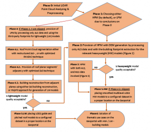
Figure 1: Phased flowchart of the overall methodological approach

geometries and by densities of sets of buildings. Probably two key types of the mentioned urban configurations are high-rise buildings of city downtowns and other central districts, on the one hand, and low-rise buildings of city suburbs / outskirts and neighboring rural areas, on the other hand. Two methodologically different AFE-techniques outlined in the previous chapter of literature review – the High Polyhedral Modeling of buildings and the Low Polyhedral Modeling – should be applied to these two urban configuration types exclusively – HPM to high-rise building sets, and LPM – to low-rise ones. We can emphasize as a strong point of our overall R&D approach just this joint employment of these two technically different methods within the united building detection, extraction, and modeling methodology, what is resulted further in the relevant software elaboration with two different tools – Building Extraction (BE, for a case of HPM), and Building Extraction Rural Area (BERA, for a case of LPM). Some common features of both approaches and relevant software tools have been already presented in some of our previous publications, although we have not made yet an emphasis on an allocation of both HPM, and LPM within a unified workflow [1, 4, 43, 102]. Since in many cases Airborne LiDAR survey relies on existing territorial regularities of urban areas, it is often provided consequently – from city central parts to outskirts. According to this, if presenting our general approach as a phased methodological flowchart, it would be reasonable to accept the HPM as Previous AFE-Phase and the LPM – as Subsequent AFE-Phase (Figure 1):

It is shown in Figure 1, that an activity diagram combines both HPM, and LPM issues, while an input is a raw LiDAR Point Cloud (Phase 0). Analyzing & Preprocessing phase implies evaluating point densities, survey induced and filtering induced errors, as well as checking a for a point cloud proper georeferencing. Two key factors, that determine a solution to be made on Phase 1 (either HPM, or LPM chosen) are the territories of specific urban configurations, that are overlapped by .LAS files, and if the third-party (OpenStreetMap, Microsoft, etc.) footprints are available for a given area.

Phase 2 implies a provision of the phased flowchart HPM-branch by processing only ALS data with extraction of the original footprints and with generation of HW-building models, which surfaces consist of numerous polyhedral facets. The output model quality is estimated by several algorithmic evaluating parameters, and in the web-software UI (a user interface of the Detailed Viewer tool) by comparison of building surfaces’ allocation in 3D space with their neighboring Lidar points. A procedure of such evaluation is illustrated further in this text. If model quality is accepted as either good, or satisfactory, it may be necessary to go directly to Phase 5.HW, since both Phase 3 (involvement of MSL data in addition to ALS ones), and Phase 4 (a whole LPM-branch) have to be skipped in this phased flowchart scenario. Phase 3 is accomplished, if MLS data employment can substantially contribute to the quality of HPM-building models with not only precise reconstruction of their facades, but also with increasing of overall sustainability of the high polyhedral model of a building by adding supplementary facets of its minor surfaces. Phase 5.HW is also a further target, if acceptable model quality is obtained on Phase 3, and, in general, if the most of HW-models are of acceptable quality. Then on Phase 5.HW these models are place to a configured dataset to a proper location on our Geoportal. A digital elevation model is generated within the HPM branch only.

Phase 4 provides the LPM-workflow, which starts from Phase 4.1, within which surface normal determination as an initial step of roof surface reconstruction within the SaS-approach, is accomplished. It is followed by a roof point cloud segmentation either in the updated SaS-methodological frameworks, or by a segmentation provided with the optimized RANSAC-technique. Both these choices are described further in the text. Phase 4.2 represents preliminary solutions for the LPM-building reconstruction stage with our original contribution to building a matrix of roof planar segment adjacency. Phase 4.3 finalizes the building reconstruction stage by combining a building from geometric primitives extracted from a point cloud on the previous stages. If the most of LW-models of buildings with gable and pitched roofs are of acceptable quality, upon Phase 5.LW they are placed to a configured dataset of models to the Geoportal (it is defined further in this text). If the quality of the LPM output results is not acceptable, the HPM-pipeline is attempted as an alternative, and a repeated workflow starts again from Phase 2. The LPM branch of our overall methodological approach does not support the DEM generation functionality.

An accomplishment of the overall approach is normally finalized on Stage 6 by solutions with HW- / LW- models of the thematic use cases on the Geoportal, what is briefly illustrated further in our paper.      

Optimal LiDAR point density values that were empirically defined for processing techniques involved on Phases 2 and 4 are between 5 and 140 ALS points per sq. m. If MSL / UAV-LS data are added to our HPM AFE-pipeline, these data are thinned out to acceptable values by sophisticated thinning algorithms, although Phase 3 deals with up to several hundred of MSL points per sq. m.

A sketch of our core algorithmic workflow of High Polyhedral Modeling is depicted in two flowcharts below (Figures 2, 3).  It has been elaborated within the frameworks of the integrated Building Extraction (BE) / Change Detection (CD) / Digital Elevation Model-Generation (DEM-G) pipeline of ALS / MLS / UAV-LS data processing. The complete algorithmic workflow depicted on the first flowchart (Figure 2) intends to extract both topographic surface, and urban features from ALS data arrays only, what corresponds to Phase 2 of the overall methodological flowchart (Figure 1).

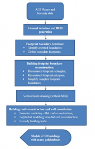
Figure 2: Algorithmic flowchart of building detection, extraction, and reconstruction within the HPM frameworks, while MSL data processing is not involved [102, p. 166]

3.2.  High Polyhedral Modeling for Building Extraction – Heavyweight Models

Thus, a flowchart depicted in Figure 2 does explain the thematic content of the Phase 2 block of the phased methodological diagram (Figure 1). Detailed consideration of this phase shows that initially the necessary preprocessing is accomplished within the first algorithmic block (ALS Range…). Then all Lidar points are separated for those, that belong to ground, and for other ones, that belong to non-ground features (block Ground detection…).

Delineation of the original building footprints (as a valuable alternative to the third-party ones) is a crucially important component of the HPM pipeline (Phases 1-3, 5 Figure 1), and it is completed within the third block of the HPM ALS algorithmic flowchart (Footprint boundary detection) – Figure 2. The footprints extracted are a self-sufficient entity for a whole HPM-ALS pipeline of Phase 2, and the following block (Building footprint boundary reconstruction) predefines modeling of a whole building, but the preliminary to this reconstruction procedures of footprint boundary optimization and more precise allocation have to be accomplished according to three sub-blocks of this block indicated by the bulleted records (Reconstruct footprint rectangles, Reconstruct footprint polygons, Simplify complex footprint boundaries). Thus, through processing upon this fourth algorithmic block building footprints are determined as quadrangles, rectangles, or routine polygons. Then “pretended” walls are arisen from the defined boundaries of footprints (Vertical walls…block).

With the next algorithmic block (Building roof reconstruction….) the rooftops of buildings may be raised from these delineated boundaries and then corrected by the data of the same ALS point cloud used upon all five previous blocks of this flowchart (Figure 2). A building which has a flat roof is modeled in prismatic geometries (a bulleted record for a subblock Prismatic modeling – flat roof reconstruction). If a building possesses some complicated shape of its rooftop, it is modeled as a polyhedron (a bulleted record for a subblock Polyhedral modeling: non-flat roof reconstruction). As it was already mentioned above “HPM” means that initially reconstructed building facets consist of many polyhedrons and represent HW- models contrary to that solution (“LPM”), while LW-models can consist of few polygons only. According to the understandable reasons, HW-models are normally constructed and visualized as comparably heavier entities (from 20 to 150 thousand of points are processed per model). Thus, mandatory smoothing and noise removing should be evidently provided. For these aims our original contribution to a Delaunay refinement algorithm [100] has been employed. The corresponding “covering Delaunay TIN” is involved to algorithmic sub-blocks Polyhedral modeling: non-flat roof reconstruction, then – to a subblock Remedy building walls.

In the presented way we have just introduced the thematic content of Phase 2, which is in our methodological flowchart (Figure 1). As it has been emphasized above, if the output model quality (the finalized algorithmic block Models of 3D buildings with many polyhedrons) for the results based on the ALS data only is not acceptable Phase 3 of the phased methodological diagram should be involved.

The initial input data for the HPM ALS / MLS / UAV-LS    algorithm, which is core content of Phase 3, and which flowchart is presented in Figure 3, are as follows:

• The points that have been received by ALS (x, y, z coordinates and RGB color attributes) Lidar survey. It is geoprocessed as a set of 3D point layers;
• The points that have been received by either MSL, or by UAV-LS scanning, or by both (x, y, z coordinates and RGB color attributes). It is also geoprocessed as a set of 3D points layers;
• The regular earth surface (a grid layer – a DEM), that has been generated upon the first algorithmic steps with existing gaps within those locations, where ground data are absent, is also accepted as an initial input for further processing;
• The smoothed regular earth surface (a refined grid layer) as a DEM with gaps removed by chosen algorithmic procedures, therefore this surface is a continuous one.

On the base of points’ distance to a smoothed DEM the HPM ALS / MLS algorithm of Phase 3 (Figure 3) separates raw Lidar points into two categories, as it is done in those procedures completed by the HPM ALS algorithm of Phase 2 (Figure 2). The first one contains the ground points that form “a ground level of this building footprint”. The second category contains non-ground points that are clustered with this building footprint. The relevant point cluster normally represents a single building or a tree. The upper blocks of the ALS / MLS algorithmic flowchart display all preliminary pre-processing / classifying steps that are provided (Detection of non-ground and ground points; Pre-processing; Classifying based on points’ coplanarity; Delineation of preliminary footprints) (Figure 3). On further classifying steps any Lidar point is assigned to be either a building point, or a non-building one. According to this binary labeling the primary footprint extraction is implemented as a technique of obtaining building footprint polygons from ALS data exclusively, thus this procedure is completely the same in both algorithmic workflows (Figures 2 and 3). This operation is normally performed in two steps: generating preliminary footprints from existing grid gaps and extracting the exact finalized footprints from these preliminary ones. The preliminary footprints are extracted as No Data holes in a grid. It is reasonable to examine this extraction slightly more in details in comparison with other components of both algorithmic workflows. It is the content of the flowchart block ALS footprint (preliminary, exact) model (Figure 1). The following modeling-extracting steps are performed for preliminary footprints:

• An initial grid is divided into the blocks of a size not more than 4’000’000 cells. Neighboring blocks possess an intersecting part of the size, that is specified by the Max building size After this step each building block is processed detachedly;
• Each cell either is marked as a ground (where the surface grid contains some value), or not classified at all (where a grid has no data);
• Thus, assuming expandCount = (params-> MaxCorridorSize / (2 * cellSize) + 1; We expand the ground class on expandCount units in the urban metrics. Afterwards we expand No Data class on expandCount; This step separates single long buildings in their ribbon sets connected by urban corridors;
• Assuming expandCount = params-> MaxCorniceSize / cellSize + 1, we expand No Data class on expandCount to join semi-attached buildings;

Figure 3. An algorithmic content of Phase 3 of the phased methodological flowchart (Figure 1) – building detection, extraction, and reconstruction                                       within the HPM frameworks, when both ASL, and MSL data are used

• Consequently, we find gaps in a grid through 1)-4) and each of these gaps retrieves its own index. In this way, only those holes that are completely isolated, i.e. surrounded by the bare ground, are expected to be found;
• Afterwards, we should check each of gaps and store only those ones, that possess an area larger, than a certain threshold value specified in the preferences;

Thus, we obtain the areal boundary for each gap considered to be a preliminary footprint. The exact footprints are generated proceeding from the preliminary ones and from some supplementary information of this point cloud. For every “exact footprint” several following steps are provided.

• All the points delineated by a geographical extent of some boundary (its size is the algorithmic parameter, which is equal to MaxCorniceSize) are selected for processing;
• All Lidar points, that are above the ground surface, but lower than 2 m above are classified as the ground points;
• After this, through all points the triangulated network is being built. Within this network all edges, which possess at least one junction, that has been classified as the ground, should be deleted.
• This triangulated network is divided for several connected segments by removing all the edges, that are longer than All network segments that have an area more, than a minimal building footprint value (that is the algorithmic parameter), are assumed to be the footprints or building parcels;
• The next algorithmic step is filtering trees. There are three possible customized options in this procedure:

1. Tree filtration is turned off. In such a case this step is skipped;
2. Applying preliminary filtration. The information about trees or non/trees is obtained from the classified source Lidar file;
3. Applying to a point cloud our own classifying technique.

Upon this fifth algorithmic step, the triangulated network is normally built through all points that are located inside those previously created footprints (preliminary ones). Then all vertical edges associated with this extracted from a point cloud entity are removed. The edge is supposed to be vertical, if its horizontal slope is more, than a certain threshold – a minimal angle, that is a parameter of the algorithm. After this procedure completed, the triangulated network is partitioned for several connected components. Then the points from components, which area is less than MinBuildingPartArea, are designated as non-building points, and are removed from the footprint entity.

• At the next algorithmic step, a new triangulated network is built through the points that belong to building parcels only; moreover, those vertical edges, which 2D length is longer than MinWallSize (the key algorithmic parameter) should be removed. The jointed polyhedrons with their aggregated areas, which are more than minimal building parcel area, are accepted as the footprints.
• The final step of the exact footprints extracting is expanding of their preliminary templates obtained through 1)-6). This step is necessary, since some building and infrastructural units, that are above the ground or above other constructive parts, are filtered out on the previous algorithmic step. To expand a footprint template the iterative algorithm is applied. Upon every step of this algorithm those points, that have not been classified yet as a constructive building or the ground, are classified as a building in a case, when this point is nearer to a footprint, than some assigned threshold distance. Afterwards, all these points are added to a footprint, and the new expanded footprints are built as an external boundary, that crosses all points that were previously classified as building points.

After all exact footprints are extracted from the preliminary ones (footprint templates), each of them should be checked for intersection with a source preliminary footprint so that to avoid topology errors. All those ones that do no intersect have to be filtered out. At the end of the block ALS footprint (preliminary, exact) model all Lidar points, that are located inside the examined parcels, and that do intersect, should be marked as the building points (in this way avoiding an extraction of other footprints that may be located within the same area). Finally, we accept the exact footprints as some planar parcels. The algorithmic step of their refinement is completed at the next algorithmic block A complete ALS model. The procedure of the planar segment refinement is quite lengthy therefore it may be a subject of description in another text. Thus, summarizing all stated above, we should emphasize that a preliminary footprint is an entity, which is extrapolated through the ground points without filling corresponding gaps at perspective footprint locations.  The exact footprints are built proceeding from preliminary ones and by providing outlined algorithmic steps.

Just as in the HPM ALS algorithmic pipeline of Phase 2 (Figure 2) our update of a Delaunay refinement algorithm has been employed. The relevant “covering Delaunay TIN” creation is completed in the flowchart blocks of Planar segment refinement, Footprint model / Pyramidal model, A complete ALS-model (Figure 3). All algorithmic blocks mentioned above are provided for processing ALS data only and reconstructing only HPM-building roofs and some other supplementary constructive components.

 The HPM AFE results of both Phase 2, and Phase 3 obtained by the Building Extraction software tool is a set of building models, each of them, as a rule, consists of few façades. The textures may be placed on these façades. Each of these heavyweight models is stored by .OBJ /.B3DM (“Batched 3D Model”) /.KML formats, but in the relevant software environment the main inner format is .OBJ. Each HW-model has its six mandatory components:

• A footprint. It represents a smoothed 2D polygon, which allocates a building footprint;
• A pyramidal model that is not draped. This model consists of several horizontal polygons at different levels. From every layer a vertical building wall is dropped to the previous level. From the lowest level the walls are dropped to the ground level;
• A draped pyramidal model. This model is the previous one, but each of its polygons has a texture. ALS points are only used for creating textures due to quasi-horizontal polygons (“roofs”). As far as creating textures for vertical polygons (“walls”) is concerned, preferably the MSL points should be applied to support a desirable level of details (LOD);
• A complete model. This model is generated either by using of the detailed TIN techniques on the Airborne Lidar points only (A complete ALS model block – Figure 3), or by combining ALS results with the wall segments reconstructed on the base of MSL data and obtaining a combined model (ALS-MLS models merged);
• Texture Mapping: draping textures on an ALS-MLS merged model;
• Detailed and precise reconstruction and visualization of the finalized model with 3D building façades.

The reconstructing operation for building façades is exposed by the MLS model completion block of the flowchart in Figure 3. The latter provides a necessary “noise clipping” procedure for building wall surfaces.Since if the distance threshold value, that means a metric length from a given Lidar point to an extracted façade, is either lower, or approximately equal to the points’  density value, the reconstructed planar surface may be a set of outliers, e.g., small peaks. Exactly in this case a procedure of noise clipping should be provided.

As it has been aforementioned already, the ALS models, on the one hand, and the MLS models, on the other hand, are merged at a certain point of the flowchart in Figure 3, just after the Planar segments refinement and the MSL model completion blocks, and before the Texture mapping block. This block means the penultimate  algorithmic step – texture draping on a merged model. In this way, for each modelу component, every polygon in the pyramidal model, the textures are being built. All those Lidar points that are located near the texture extent can be found. These points are projected on the roof / façade plane, and the coloring of the texture pixel is initiated.  All predeccor algorithmic blocks in the flowchart of are ended by the Detailed 3D reconstruction of building façades one. Finally, the results are being delivered into .OBJ and .B3DM formats, and a composite high polyhedral model can be displayed by the relevant visualizing software tools developed by the authors (Figure 4). It can be seen, that the HPM AFE  results in numerous polygonal segments, which represent quite a rough surface, only while zoomed in. Even a model of numerous polyhedrons can be impressively displayed by our provided visualizing technique.

After completing the HPM-algorithmic workflow, a user obtains building models for display either in the ElitCore desktop application, or in the web-based  ELiT (EOS LiDAR Tool) Viewer with three levels of detail (LODs): LOD 0 represents a model footprint as its projection on the plane;  LOD 1 is a 3D object that exposes a building as a set of prisms – a pyramidal model;

LOD 2 displays smoothed multilevel models in minute details (Figure 5). We have expressed an idea in the introduction to this text, that the composite (ALS / MLS-UAV-LS) model of extracted features may be the most effective one, primarily, with respect to user’ various applications in many industrial domains. Such a typically smoothed multilevel model of LOD2, a HW- model, may be like follows in the ElitCore desktop UI (a user interface) (Figure 5). Thus, despite visualizing rough building surfaces, if significantly zoomed in, while applying to the LiDAR data intentionally selected and refined by the ALS / MLS algorithmic workflow on Phase 3 of the overall methodological flowchart (Figure 3).

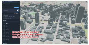
Figure 4: Results of the HPM ALS / MLS workflow displayed in the viewer of the web-based applications – building roofs of many polygonal segments. The downtown of New Orlean, USA (a dataset from the EOS LIDAR Tool landing page: https://eos.com/eos-lidar)

Figure 5: Model of one the historical buildings from the Ottawa downtown in the ElitCore desktop user interface

The presented methods of the HPM on Phases 2, 3 is a completely original AFE-methodology elaborated by the authors. It has been implemented in Building Extraction (BE) (Figures 4, 5) and Change Detection (CD) (Figure 6) functionalities of our both desktop, and web-based applications.

3.3.  Low Polyhedral Modeling for Building Extraction in Rural Areas – Lightweight Models

3.3.1.     Common issues

Oppositely to the High Polyhedral Modeling technique our another AFE-approach is the Low Polyhedral Modeling method,

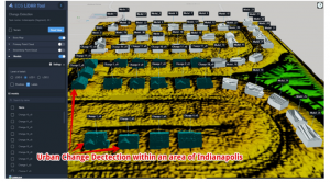
Figure 6: Results of the CD functionality application: new buildings (labeled as Changes in dark green color) as urban changes that appeared within one year’s time. Models of both new, and old buildings (labeled as Models in light grey color) are placed on a DEM generated. An area of Indianapolis, Indiana, USA (a dataset from the EOS LIDAR Tool landing page: https://eos.com/eos-lidar)

which is a procedure of planar segmentation and classifying clustering of Lidar points. That corresponds to Phase 4 of the phased methodological flowchart and to all its inner constituents (Phases 4.1-4.4) (Figure 1). This approach attempts to determine for each Lidar point either its planarity, or non-planarity. For solutions on the roof segmentation stage we have employed both SaS [35, 37] separation of parallel and coplanar planes, and RANSAC [62, 63, 65] clustering technique (Phase 4.1). Some original optimizations have been applied for each of these two methods of segmentation. For clustering and plane segmenting with the SaS-methods the more effective workflow structuring has been provided, that is described further in this text.  While for RANSAC – a particulate improvement of the candidate plane selection has been introduced. On the preliminary building reconstruction stage (Phase 4.2), the SaS-methodology has been enhanced by the innovative technique of building roof plane adjacency matrix and the neighborhood selection (Phase 4.2).

On the finalizing building reconstruction stage theoretical basics of the PolyFit [65] have been effectively implemented in the applied solutions with web-software (Phase 4.3).

We have mentioned already, that initially the LPM is intended to extract low-rise buildings in either rural areas, or city suburbs.  Nonetheless, it has been successfully applied to various urban configuration even within central parcels of the large city areas. Because of the segmenting / clustering procedures that drastically decrease a number of polyhedrons as constituents of a model extracted, such model is titled as ”low polyhedral” one. We emphasized already, that these models are extracted, reconstructed, and visualized as the LW-models (approximately from 5 to 40 thousand of Lidar points processed per one entity). After completion these models are composed of only few polygonal planar segments. Models are reconstructed in this way, and each of them represents a lightweight modeled feature as a final solution.

 Building reconstruction of low-rise constructive features is implemented as a finalizing procedure of building modeling (Phase 4.3). This algorithmic stage begins with the adjacency matrix of roof plains generation, that exposes the connectivity of the delineated planar segments. Our original contribution to the formation of the plane adjacency matrix is described in the one of the following subsections of this text.

Both roof interior, and exterior vertexes are determined. Topologically consistent and geometrically correct building models are obtained through implementation of the extended boundary regularization approach. The latter is based on multiple parallel and perpendicular line pairs, and just this approach expedites an achievement of the reliable building models.  The model precision can be effectively tuned, despite it understandably still depends on the data precision. In any case the model precision may meet the strict customer requirements. The low polyhedral model implemented corresponds to LOD 2 of the City GML standards [17, 19, 22]. The following visual presents the main content and some attribute information of this LPM algorithmic result in the interface of our cloud-based software (Figure 5). A number of acceptable models among all LW-models generated is a criterion of going either to Phase 5.LW  with model output to the Geoportal, or Phase 2 so that to repeat processing and modeling by shifting to the HPM branch (Figure 1).

Figure 7: The LW-models of buildings with gable and pitched roofs (pointed to by grey arrows) in a small town. The city of Lubliniec, Poland                                                         (a dataset from the EOS LIDAR Tool landing page: https://eos.com/eos-lidar)

3.3.2.     Enhancing SaS-segmentation by restructuring its pipeline

It is an initial content of Phase 4.1 of the phased methodological flowchart (Figure 1).

1. To Save removed points for further processing. The points removed on the previous step are added to those points, that have not been assigned to any cluster.
2. To Assign unclassified points to the clusters. An addition of formerly unassigned points to a proper cluster might be a key procedure for various configurations of roof individual segment delineation. Some of these points might not be assigned to any cluster due to noise impact (a roof segment under a tree), or because of neighborhood nonplanarity on a seam between two or more roof slopes.
3. To Separate parallel planes inside each cluster. Surface normal vectors are being clustered initially. A clustered entity with the same normal vector is created. Thus, primarily a cluster is a set of planes, and a distribution of parallel planes into separate clusters inside this primary cluster takes place just on this step. The parameter D (from Item 1) is being computed for all points, and the latter are clustered. The output is a set of planes with the same normal vector, but on the different distance from the center of coordinates.
4. To Split coplanar clusters using the Voronoi neighborhood. A segmented plane may combine those roof segments, that are not connected spatially, but other segments are between them. Such coplanar planes are separated on this step. Commonly, these Items 5 and 6 correspond to the Separation of Parallel and Coplanar Planes step in [37].
5. To Remove small clusters (optionally – using the Voronoi neighborhood). Small area segments can be left after separation of parallel and coplanar clusters. These features should be eliminated as the noise and clustering errors.
6. To Remove the near-vertical clusters, because the modeling technique does not use them due to their unreliability.

It is reasonable to emphasize intentionally that the Phase 4.1 initial content steps 1-6 can be completed only for a point cloud of some robust density, that may lie within the earlier mentioned range of 5-140 ALS points per sq. m.

3.3.3.    Providing RANSAC enhancements

It is another content of Phase 4.1, and the optimized RANSAC-technique can be employed for a roof plane segmentation as an alternative to the SaS-approach, which has been somewhat restructured in comparison with an original issue in Item 1-6 in the previous subsection. We have already mentioned in the reviewing section of this text, that the RANSAC algorithm is able to extract a manifold of geometric primitives with different types of their shapes. RANSAC can deal with large number of outliers in the initial data, since this resampling method uses the smallest number of points necessary for estimation a given geometric primitive [62-64, 89, 103, 104]. Thus, the corresponding geometric primitives are obtained, if they approximate definite majority of points.

Some debatable issues present in the initially attempted SaS-segmentation, which appeared to be drastically sensitive to various outliers in the point clouds like, e.g., overhanging (above a building) trees. Because of this and due to the Lidar induced errors usually caused by sharp changes in the heights for the points belonging to the same feature, we have finally employed RANSAC with some editing of its general scheme. It may assist in meeting the challenges mentioned. For example, when the most points do not have the planar neighborhood, while the normal surface vectors, that are nonetheless found for the point minority, are located randomly, and this does not allow to delineate a corresponding point cluster for plane extraction.

In the outlined case, the RANSAC shape extraction strategy gives an opportunity to delineate a planar segment even facing the challenges mentioned, because the sufficient condition is a randomly drawn point set, that can be quite feasible for this drawing, and employed then for constructing planar segment primitives. 2D planar points and 3D non-planar points can be separated ones from others using this technique. Figure 8 shows the example of a building model, which planes have been segmented with the optimized RANSAC from a point cloud with numerous outliers. Then this model has been refined and efficiently reconstructed, and even an overhanging tree, that is comparable in its size with a building, has been removed.

We have selected a following number of the basic RANSAC enhancements practicable for the ALS point cloud segmentation and implemented it in the relevant algorithmic pipeline embedded in our web-based software:

• Number of iterations upon the planar facet-candidate selection is not a constant, but it depends on a qualitative value that is the Best Current Candidate Plane Index (BCCPI), a total number of Lidar points involved, and number of attempts completed yet. The purpose of the BCCPI value introduction is somewhat resembling to the RANSAC “score of the shape” [63], that also provides formalized estimation for the candidates of planar facets.
• Any BCCPI value is defined as number of points within the delta-neighborhood of a plane minus the “penalty charges” for the point dispersion. Thus, the less is point scattering from a detected plane, the higher is a qualitative

Figure 8: A building model reconstructed from the plains detected and segmented by the optimized RANSAC. A model is visualized by the Matplotlib python library. A building located in the city of Lubliniec, Poland

value of a candidate plane; the bigger is the scattering, the lower is a value mentioned. This technique reasonably allows to prefer those candidates, which approximate well even a relatively small point cluster, but not those random plains, that cross a whole extent of a model and overlap a big number of points in its delta-neighborhood. It is quite significant especially for the gable roofs with minor angles between its two slopes, or for pitched roofs with small angles within each pair of this roof slopes.

• The adaptive alteration of the rules due to the plane candidate “penalty charges” for a size of point dispersion. The relevant procedural scheme may be evident: if after a certain number of iterations, a reasonably acceptable plane-candidate has not been extracted yet, a decrease of “penalty charge” is introduced, so that at least a less acceptable plane-candidate can be detected and chosen. It may be wise to start by setting the high BCCPI values at the initial stage of the plane-candidate selection, then gradually decrease these values, if processed point clouds appear to possess much data noise and numerous outliers. Specifically, such approach gives an opportunity to detect quite precise roof slopes in point clouds with low data noise, but instead, a threshold for the BCCPI values may be intentionally decreased for overlapped strips resulted upon the airborne laser scanning, when a flight changes surveying direction.
• According to the improved RANSAC basics the point sampling for a plane-candidate may proceed from a whole point cloud with associated normal vectors, and the technique output is a set of planar primitives with corresponding point sets [105]. Such procedural content may cause some significant inaccuracy itself, while attempting to detect a plane, which may cross a whole cloud as explained above. Instead, we introduce the point sampling from a randomly chosen limited neighborhood. On the one hand, with this selection we still have the chances to approximate a big planar facet, if one does exist, on the other hand, we are expected to approximate some relatively small planar segment precisely enough, if a big one does not actually exist. If sampling neighborhood reduction is not provided, the probability that all three points, a point triple, would approximate (a key criterion of plane detection) one small planar facet has a low value.
• A point triple should be checked for the degeneracy: if an area of their triangle is too small, then the probability of processing error is high enough, and the whole computation cycle may fail. Therefore, such triple is rejected, and another one is sampled.

The overall structure of our optimizations of RANSAC is presented in the following Algorithm Pseudo-Code (Figure 9):

1. Main cycle:

working_set := input_points

result_planes := []

WHILE len(working_set) < threshold:

  plane_parameters, remaining_points := fit_plane_ransac(working_set)

result_planes.append(plane_parameters)                                            working_set := remaining_points

 

2. Selecting candidate plane function (fit_plane_ransac)

best_sample_quality := 0

best_sample_size := 0

best_sample := None

iteration := 0

WHILE probability(best_sample_size, points, iteration) < quality_threshold:

  IF iteration >= iteration_threshold:

    reduce_dispersion_influence_on_quality_estimation()

    IF check_quality_limit_reached()

       BREAK

    iteration := 0

  p1, p2, p3 := select_candidate_points(points)

  iteration := iteration + 1

  IF NOT check_candidate_area(p1, p2, p3):

    CONTINUE                 

  candidate_sample, candidate_quality := get_best_candidate(p1, p2, p3, points)

  IF candidate_quality > best_sample_quality:

    best_sample_quality := candidate_quality

    best_sample_size := size(candidate_sample)

    best_sample := candidate_sample

3. Assessing candidate quality function – BCCPI value (get_best_candidate)

plane_parameters, sample_points := fit_plane(p1, p2, p3, points)

points_distance := get_distance_to_plane(plane_parameters, sample_points)

distance_dispersion := mean(points_distance)

quality := quality_influence * (len(sample_points) / len(points)) + (1 – quality_influence) * (1 – dispersion / plane capture_distance)

Figure 9: The Pseudocode of the optimized RANSAC

It has been determined that the optimal initial value of quality_influence may be 0.4, while the iteration step in reduce_dispersion_influence_on_quality_estimation is 0.1.

3.3.4.    Optimizing SaS-reconstruction by Voronoi Neighborhood

One of our key contributions to the SAS-methodology corresponds to Phase 4.2 of the phased methodological diagram (Figure 1). It consists in the refinement of the optimized adjacency matrix obtainment on the preliminary stage of building reconstruction. This matrix is the most significant issue for the delineation of the adjacent planar segments in the model generated. Thus, we have enhanced the SaS-workflow by the extensive use of the Voronoi neighborhood for computation of the roof segment cluster adjacency on the building reconstruction stage. Although the authors of the original workflow referred to the Voronoi diagram only on the point cloud segmentation step – the Voronoi neighborhood V_p has been employed for the surface normal computation only [37, 76]. Applying to the Voronoi diagram on the building reconstruction stage, we remove both horizontal, and vertical gaps in the processed data, as well as mitigate the nonhomogeneous point density of a primary point cloud.

The Voronoi diagram has been applied for the roof cluster adjacency determination and for separation of coplanar clusters, while the limited Voronoi diagram has been used for avoiding the side effects of the cluster adjacency determination. Also, the Voronoi diagram has been applied for the reliable identification of some traditional architectural constituents such as building awnings and or building overhands [102].

The Voronoi neighborhood for the roof cluster adjacency determination means the obtainment of the planar segment optimized adjacency, on the condition that these segments are preliminary delineated. The authors of the SaS-methodology use the Voronoi diagram while providing eigenvalue analysis, and each point of neighbors are being delineated. Nonetheless upon computing the cluster adjacency these authors apply a routine distance between all pairs of points using the following formula [37, P. 1562]:

d (P,Q) = min (d (p_i,q_j)) ∀p_i ∈ P; ∀q_j ∈ Q,                    (1)

where: d(p_i,q_j) is a distance between any pair of points p_i and q_j , which belongs to two different  clusters P and Q correspondingly. The problematic issue of the SaS-approach like presented with (1) proceeds from a case of nonhomogeneous point cloud density that is a subject for clustering and segmenting.  E.g., a sparse point cloud, which is also worsened by the faults of surveying technique, reasoned the case, according to which clustered points appear far from the boundary of a cluster. In such a case a distance value (from (1)) fails to be proved, if it is checked by a threshold parameter. Consequently, this may be a reason for the errored adjacency determination and for the consequent   wrong model reconstruction.  Nonetheless, it may be not so wrong to conclude, that because there are no Lidar points between two delineated planar segments, which would belong to other clusters, these two segments are sooner adjacent, than not and their seeming “non-connectivity” might be caused by the gaps and outliers in Lidar data only. This problem may be resolved by the adjacency determination with the Voronoi neighborhood.

The possible solution can be based on the following assumption. Even in a case, when two points lie far from each other, and there are no those points between them, which may belong to the third cluster (besides a given pair of clusters), and the Voronoi cells of these two points have common edges, then this pair of points can be determined by their Voronoi neighbors. In another case, when there are points of one more cluster between a given pair of points, these points are not considered as the adjacent ones even, if they pass a comparative test by applying a threshold parameter large enough.

On the base of all mentioned above and referring to an existing relevant example [106], we assume to consider as adjacent ones only those clusters, which points are neighbors within the Voronoi neighborhood. The only criterion is a case, when their Voronoi cells possess a common edge. Thus, we both solve a problem of data scarcity, gaps / outliers, and find a solution for a sparse point cloud. What is more, we get rid of a necessity of the enlarged threshold value introduction, but implement its definition by interpolating technique instead, since this value should be both big enough (not to remove the actual adjacent clusters), and small enough (not to define non-adjacent clusters as adjacent ones). In this way, we can significantly increase the applicability of our approach, and decrease its narrowness, e.g., when it strongly depends on point density and on the equitability or at least on the similarity of spatial distribution of the points that belong to two clusters. Moreover, the search of the Voronoi neighbors can be completed faster with such approach, because each point has a computed list of neighbors to be checked for their spatial acceptability. Thus, the overall algorithmic efficiency can be increased. It is only the first aspect of the overall LPM optimizing. The second one, that is not a less important solution, is introduced in the following paragraph.

While arranging the matrix adjacency in the frameworks of the SaS-technique, we define the distance between two clusters of planar points d (P, Q), as the minimum of all point possible combinations between two clusters distance (1). Then, m =| P | is a point number in the first cluster, and n =| Q | – a point number in the second cluster. Hence, a whole number of possible combinations to be computed in such a case is the m · n value, the product of the point numbers.

Figure 10: A lightweight model of a building with the pyramidal roof and an outhouse reconstructed at the ElIT Geoportal in the location of the city of Lubliniec, Poland

At this algorithmic step we suggest an alternative solution: to extend each of two clusters of planar points up to their mutual intersection, while a relevant linear segment of the cluster intersection is generated. Then we compute the distance between two clusters as the minimal distance of all possible measured combinations between points belonging to each of two clusters, from one side, and this linear segment of a cluster intersection, from another one. The statistical significance of difference between two mentioned values can be estimated. A combination number in this case becomes substantially fewer: the m + n value only, the sum, but not the product. It defines the significant simplification of the overall LPM algorithmic complexity from the quadratic complexity O (n²) (a case of the point product that defines number of combinations) to the linear complexity O (n) (a case of the point sum, that defines number of combinations). Decreased complexity provides the overall enhancement of the LPM-algorithmic efficiency.

It is evident, that the better a roof segment matrix is optimized, the more sustainable number of geometric primitives (e.g., vertices) is necessary for the robust building roof reconstruction. The introduced update of the adjacency matrix computation provides the definition of some threshold levels between two clusters of coplanar points within a footprint boundary, which is accepted as a geometric analogue of the roof edge. These clusters should never intersect, and this circumstance causes an indefinite exit of computing guaranteed, if the traditional approach is attempted to provide. Otherwise, the updated LPM technique, in its turn, completes the modeled topological sustainability and geometric correctness of a building footprint and of its roof as shown in Figure 10. It displays a model example from a fragment of one from modeled CityGML LOD2 locations placed at our internet-resource – ELiT (EOS LiDAR Tool) Geoportal (http://elit-portal.eos.com/). The presented lightweight model has been selected for display, just because the relevant point cloud possesses quite a few non-intersecting planar segments, that is why the routine SaS-algorithm of reconstruction has failed while processing this data, but its update has succeeded – Figure10.

3.3.5.    Implementing the PolyFit approach

Phase 4.1 and partially Phase 4.2 examined above deal with the point cloud segmentation stage in an overall processing workflow. Correspondingly, our prime LPM-concern has been a set of the roof segmentation operations, as it has been previously discussed for these two phases of the methodological diagram.  Phase 4.3 provides the finalized stage of building modeling – its reconstruction, while Phase 4.2 grounds some substantial premises for it. We consider the urban feature reconstruction stage as presentation of building geometry and topology within a certain LOD with a defined number of feature segments.  That is why we have attempted to implement in Phase 4.3 one of the most interesting among other relevant theoretical technique – the polyhedral (polygonal) surface reconstruction (the PolyFit approach already mentioned in the literature review) [65, 107].

Figure 11: The PolyFit page selected among a list of other AFE-techniques in the menu TOOLS of the web-based software interface

This approach demonstrates, that reconstruction of geometric primitives from a point cloud can be treated as a binary labeling problem (what is, by the way, close enough to “global solutions” in the point cloud processing [87, 91]).  The method proceeds from the hypothesizing and selecting strategy and provides intersecting the building planes already segmented, then seeking for a necessary combination of intersected planes and getting a manifold polygonal surface model. Since in its segmentation stage the method is strongly based exactly on the RANSAC algorithm for plane detection, then by enhancing RANSAC plane primitive extraction and refinement, what has been introduced in this text above, we understandably contribute to making the PolyFit solution more robust.

Therefore, constructing a whole pipeline for the PolyFit implementation in our web-based software, we attempted to employ on a relevant segmentation step both the original advances of the SaS-approach, and possibilities of enhanced RANSAC. Thus, the PolyFit appears to become one more AFE-option in the relevant menu option of our web-software package (Figure 11).

4. Results: Software Elaborated for AFE Purposes

The applied software solutions, that can be elaborated on the base of the presented multifunctional methodological approach to the generation of heavyweight and lightweight AFE-models (Figure 1) can be introduced as the robust results of this research. These software solutions are completed with the functionalities, which can provide the efficient support and realization of all three groups of advantages referred to above.

4.1.  Desktop and Web-Based Applications

The ELiT (EOS Lidar Tool) Web-Based software is both a separate web-based (network) generator – ELiT Server (a landing demo-page available at https://eos.com/eos-lidar/), and an integrated component of EOS Platform-as-a-Service software – ELiT Cloud. The latter is the basis for ELIT Geoportal – a type of web portal used to find, access, and process LiDAR geospatial information, both primary, and resulted one, as well as provide the associated geographic services (display, editing, analysis, etc.) though the Web (http://elit-portal.eos.com/). Few examples of the ELiT Server interface have been already presented above (Figures 4, 6,7, 10, 11).

The congeneric to these two products is our desktop ElitCore package, which possesses even somewhat broader functionality, but can produce only the heavyweight polyhedral models (Figure 5). The Building Extraction functionality implemented in the standalone ElitCore provides detection, extraction, and reconstruction of heavyweight models according to our general methodological workflow of the HPM AFE (Figure 1) and its algorithmic content of Phases 2 and 3 (Figures 2 and 3). It normally results in a DEM (“a bare ground class” delineated from an initial point cloud) and a set of urban features which are the discontinuous objects.

All three mentioned software products are based on the sophisticated HPM / LPM solutions based on those complicated algorithms for Lidar data processing that have been introduced in the previous section of this text. Both ELiT Server, which has been implemented as a distributed information system, and ELiT Geoportal usually operate from the Web browser installed on a user’s workstation.

ELIT 3D city models as many other 3D models appear to be predominantly used for display; however, they are being increasingly employed in number of subject areas and for a large range of tasks beyond the visualization. In our previous publications, we sought to understand and present several use cases regarding their presentation not only on the ELiT Server, but also on the ELiT Geoportal with further utilization of these City GML LOD1 models for some tasks within and beyond model display [4, 102].

Our web-based software implies provision of the following ELiT tools as the functionalities of the distributed information system (these tools are shown in Figure 11 above):

• The Building Extraction (BE) tool (a sub-page Building Extraction of the Tools page – Figure 11) provides the HPM building detection, extraction, and reconstruction through various sub-procedures pursuing the final sub-procedure of building reconstruction for high-rise buildings, preferably in city downtowns. Thus, the BE-functionality accomplishes the generation of heavyweight models, which have been already grounded and presented above (Figures 2-4, 6). The building extraction functionality is that option, according to which any single building construction may be detected, extracted, and reconstructed as a heavyweight model with further visualization by the open source Cesium 3DTiles library with a certain LOD and with relevant spatial, geometric, and semantic attributes. Key components of the massive urban environment can be simulated as the heavyweight models with minor details (Figure 12);

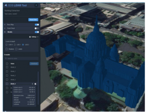
Figure 12: A historical building in a downtown of Ottawa, Canada, visualized in the ELiT Server interface

• The Building Extraction with Footprints (BEwFP) tool (a sub-page Building Extraction with Footprints of the Tools page – Figure 11) accomplishes the same HPM building extraction as the BE-tool producing the heavyweight building models. Oppositely to the previous tool, the BEwFP-functionality involves the third-party data – building footprints (global maps as Open Street Maps, ESRI Imageries, Microsoft footprints, etc.) instead of accomplishing its own ELiT footprint delineation described in 3.2 Section of this text. Normally the footprints input is an archived ESRI SHP vector file;
• The Building Extraction Rural Area tool (BERA – a sub-page Building Extraction Rural Area located on the Tools page – Figure 11) provides “a classical pipeline”, by which we implement the SaS point cloud segmentation / building reconstruction methods [37] of low polyhedral modeling introduced in Phase 4.3 of the methodological flowchart (Figure 1). According to the SaS-pipeline and to its optimization described in subsections 3.3.2 and 3.3.4 the BERA tool accomplishes the hierarchical segmentation of a Lidar point cloud, refinement, and separation of extracted planes with further building reconstruction in rural areas and urban suburbs. As it has been already mentioned above (Subsection 2.2), the generated lightweight building models consist of not so many facets, and number of points involved in a single model generation is limited by a number from five to thirty thousand. Necessary limitation may be met by adaptive thinning at the cost of modeled details, if an initial value ranks over this quantity. The correspondence of a resulted model to an initial point cloud can be visually assessed for a conclusion, if it is modeled accurately or not, and if it is allowed to go to Phase 5.LW , or it is necessary to go back to Phase 2, and provide HPM instead of with LPM (Figure 1). This quality estimation is provided with the ELiT Detailed Viewer (Figure 13). In case of acceptable quality, the point locations should not deviate on more than a certain distance threshold value from the modeled surfaces. An exact threshold is introduced, basing on the point cloud characteristics, e.g., on its density.
• The Building Extraction Rural Area Polyfit tool (BERA-P – a sub-page Building Extraction Rural Area Polyfit located on the Tools page – Figure 7) implements somewhat another algorithmic pipeline in comparison with the BERA The RANSAC optimized clustering and segmentation is used on the initial building modeling (subsection 3.3.3). The hypothesizing and sampling strategy of the PolyFit basics [65] together with its finalized reconstruction of polyhedral models is applied to concluding building modeling. Our optimization of the RANSAC segmentation described above is embedded in the relevant workflow, that fulfils the BERA-P tool. Its processing may take somewhat longer time, than the “ordinary” BERA tool does, but usually provides an increase of number of topologically correct and geometrically precise models among all output models in a dataset.
• The Change Detection tool (CD – a sub-page Change Detection, which is on the Tools page – Figure 11) automatically detects block-, district-, and city- scope alterations in an AOI selected. Changes in urban architectural morphology usually happen through city areas over some significant period, if only it is not any catastrophic event of either environmental, or social demolition. The ELiT CD tool detects locations of changes in positions and shapes of buildings and infrastructures as 3D models with additional spatial information. Usually two Point Clouds (the temporally primary, and the temporally secondary ones) are compared. It is not BERA, but the BE-functionality is the only one that is involved in preparing two resulted modeled sets. The difference between two input point clouds is computed as the BE-output of the high polyhedral modeling (Figure 6).

All those already listed ELiT functionalities are supported by the relevant web-API and by the Front-end web-interface for routine procedures of uploading, processing, and analyzing the initial data and for further downloading derivative data. The sets of modeled .OBJ and. B3DM entities (the latter are Cesium 3D

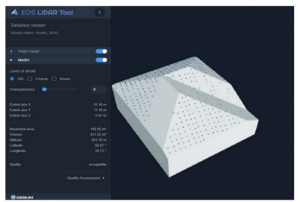
Figure 13: The Detailed Viewer Tool for examining accuracy of a lightweight model according to point cloud content

Tiles component) have to be delivered to 3D models, and can be stored and visualized in .COLLADA, .KML, and glTF formats.

According to the content of 3D Tiles specification a .glTF  is employed by .B3DM as its payload for delivering 3D building geometry. If data processed by ELiT Server, the results of all functionalities, BE, BEwFP, BERA, BERA-P, and Change Detection, are displayed by the ELiT Viewer.

• The DEM Generation tool (DEM-G – a sub-page of the Tools page Figure 11) runs a generation of a field of topographic heights making a DEM / DSM grid (Figure 17). It means we can create a gridded surface from sample data, what is commonly referred to as the interpolation. According to the contemporary basics of topographic modeling the most accurate uniformly spaced DEM matrix can be compiled directly either from photogrammetric processing of remote sensing imageries, or by processing results of LiDAR surveys [8]. In other words, a series of irregularly spaced height points are acquired, from which uniformly spaced elevation benchmarks are interpolated. A created DEM we understand as a synonym of a digital terrain model, which simulates the bare earth surface with uniformly spaced z-values of heights within a DEM neighborhood. Our automated processing for generation of a DEM of high precision provides modeling topography of various genetic types, e.g., sand-eolian (as shown in Figure 14), glacial, fluvial, volcanic, topography of human impact, etc. Results of the DEM-G functionality are visualized in ELiT Viewer by the TerrainProvider option of the open source Cesium JavaScript library (Figure 14).

4.2.  Cloud-Based Application – ELiT Geoportal

A common definition of the EliT Geoportal (EGP) as a cloud-based application has been already done in the previous subsection of this text. We already explained in one of our previous publication the necessity of a geoportal as a robust solution for the web-GIS software promotion [102]. EGP is a kind of web portal used to transform occasional visitors of the EOS LiDAR web-site into the warm leads. The EGP site can be used to find and access the derivative Lidar information and relevant services for number of thematic use cases, that can be resolved through geospatial modeling, visualization, and GIS-analysis.

Figure 14: Topography of sand dunes in Brazil visualized in the ELiT Viewer interface  (a dataset from the EOS LIDAR Tool landing page: https://eos.com/eos-lidar)

Thus, the Geoportal can be also defined as the Internet-toolbox for resolving local, regional, national, and even globalized urban problems, i.e., by performing at very different scales. A routine Web-based map-server software usually allows only backups of mapping results. Nonetheless, for various domains of Urban Studies, which can be provided with our research and modeling technique [1], we do need a Geoportal Internet-toolbox associated with a web-based Geodatabase, that would allow us to sort, query, update, and delete both different features and data associated with these features. Such architectural and structural web-software scheme differs towards its more efficiency if compared with solutions of a common case.  Within these solutions some web-based GIS application generator is developed, and it provides on the base of the routine database scheme the number of web scripts. Then it deals with a map interface and with a database, as well as with provision of interactive maps defined by a user [19, 108, 109]. Otherwise, the EGP may support an effective integration of a Web-based GIS interface with a Geodatabase chosen within a web-architecture. Spatial references and 3D regional layers are automatically chosen for a given territory. What is more, semi-automatic generation of Web 3D Scenes according to a selected AOI can be provided. Owing to this architectural scheme, series of thematic EGP use cases are provided (http://elit-portal.eos.com/): Population estimation in an AOI based on 3D building models; Energy consumption estimation based on 3D building models; Visibility analysis in urban environment for various city development scenarios’ evaluation and comparison.

5. Discussion

Choosing either the high polyhedral modeling, or the low polyhedral one with corresponding generation of either HW-, or LW-models may be selected as introductory topic of the discussion, which summarizes our research.

As explained above, in a common case, Phase 1 of the methodological flowchart (Figure 1) suggests either one, or another option according to environmental and urban configurations of a selected AOI.

There are several samples of HW-models in various datasets of large urban areas with mainly high-rise buildings, presented on the ELiT landing page as derivative results of BE and CD functionalities. From our point of view, these HW-models prove the AFE efficiency, while the relevant technique is applied either only to ALS data (Figures 4 and 6), or, especially, to combined results of ALS / MLS survey (Figure 5). The quality of HW-models obtained from ALS data can be estimated on their visual comparison with analogues in imageries retrieved from global maps (e.g., Google Maps). Normally, on the base of this comparison a decision is made within the methodological flowchart: either go directly from Phase 5.HW , or accomplish initially Phase 3, so that MLS data involvement improves the heavyweight model quality (Figure 1).

The LW-models are built exclusively on the base of ALS surveys together with input of the third-party footprints (Figure 7). The lightweight model accuracy exclusively depends on the segmentation quality and the reconstruction robustness. What is more, exactly clustering / segmenting procedures significantly define consequent LM-results. Application of the originally optimized RANSAC (Figure 9) has resulted not only in removal of a point cloud outlier caused by a tree (Figure 8), but also in predetermined appearance of a building outhouse on the reconstruction stage in a finalized model, what cannot be guaranteed with the routine approach of segmentation (Figure 10).

The comparative evaluation of optimized clustering/segmenting technique with both restructuring SaS-pipeline (subsection 3.3.2), and with enhancing RANSAC (subsection 3.3.3) has been provided on the base of several ALS data surveys accomplished over the territory of the city of Lubliniec, Poland, in 2017-2018 (Figures 7, 8, 9). Table 1 is produced to compare the modeled results of the methods mentioned. Three different values of the key RANSAC parameter from Figure 9, plane capture distance (PCD), are used in meters, evaluating the position uncertainty for each Lidar point. Consequent iterations are completed for PCD=0.1, 0.2, and 0.3. The model quality is evaluated both by a visual comparison with a processed point cloud (as in Figure 13), and by customized estimating of algorithmic parameters. Modeling warnings designate partially correct models that have some flaws.

Table 1: Comparison of the modeled results depending on clustering and segmenting method (a LiDAR point dataset on Lubliniec, Poland)

#	Method of clustering / segmentation	Pro-cessing time	Total                                         number of models	Correct models	In-correct models	Modeling warnings
1	Original SaS	8 h 45 min	934	534	289	111
2	Original RANSAC	12 h 11 min	934	577	248	109
3	SaS with restructured pipeline	11 h 24 min	934	588	243	103
5	Optimized RANSAC with PCD=0.1	15 h 57 min	934	662	167	105
6	Optimized RANSAC with PCD=0.2	10 h 42 min	934	677	147	111
6	Optimized RANSAC with PCD=0.3	7 h 42 min	934	699	133	102

Shown in Table 1 are the comparative statistics, which has stipulated the necessity development of the BERA PolyFit building modeling tool described above. The total number of models column has the same value for all records, since it is a number of building footprints obtained from a data provider for this AOI. Another almost constant column for all methods is number of partially correct models (Modeling warnings). The table shows, that for all other records the evidently best results are demonstrated by the optimized RANSAC with PCD=0.3 (Method # 6). The accuracy of the segmented roof planes follows from a selected clustering-segmenting method thus it does predefine either a success, or not on the stage of reconstruction. Therefore, this technique has been selected for the BERA-P tool. Briefly the most efficient RANSAC method according to Table 1 can be illustrated in the following way, if examining only one model (# 43) from a dataset, what from Table (1) (Figure 15).

Two different iterations of Method # 6, which present resembling results (the same number of up to seven face candidates), are illustrated, because it is the only method, that produces an acceptable number of similar results through various iterations. Lidar point as color-coded segments have ratios for each coded class. Ratio numerator is the number of break-line (non-planar points that do not belong to this segment due to the PCD value) points, while ratio denominator – planar points (they satisfy the PCD threshold). Methods ##1-6 (Table 1) have been compared with respect to similarity of various iterations like in Figure 15. Method # 6 meets criterion of the best efficiency in this respect.  The following illustration shows that this technique is the only tool (among all other from Table 1), that can provide the clustering-segmenting premises for reconstruction of a problematic roof slope, that belongs to model # 21 in the considered Lubliniec dataset (Figure 16). All other five techniques missed this roof slope.

The finalized illustration of this text demonstrates an increase for up to 27% (41 acceptable among 62 all models versus 30 / 62 ratio)  in a number of acceptable models for a small urban area in Washington, D.C. by providing Method # 6 as a software solution (Figure 17).

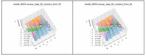
Figure 15: Two different clustering / segmenting iterations of Method # 6 (Table 1) to a point cloud of model # 43, that demonstrate resembling results

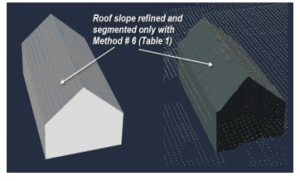
Figure 16: The roof slope pointed by arrows segmented by Method # 6 for further reconstruction. A CAD model built from a Google imagery (to the right) is compared with a point cloud with quite weak correlation for this building segment, while ELiT LW-model reconstructed is to the left

6. Conclusion

Our paper focuses on the conceptual multifunctional (functionalities of Building Extraction, Building Extraction in Rural Areas, Change Detection, and DEM Generation) approach within the AFE frameworks, that has been introduced through consequent steps of the phased methodological flowchart. In general, a workflow presented that has been completely automated for building detection, extraction and modeling by processing ALS and MLS point clouds. Two approaches of the high polyhedral modeling, and the low polyhedral one, have been proposed as two phased branches of a united overall workflow. These two modeling mainstreams have been compared on the base of their resulted models: the heavyweight models generated together with their original footprints within the HPM frameworks, and the lightweight models that employ the third-party footprints – with the LPM technique. With modeled results illustrated we have attempted to prove that the HPM branch can be appropriate for high-rise building reconstruction with either flat, or pitched roofs in densely build-up urban areas. The LPM branch – for modeling low-rise buildings with gable, or pitched roofs in either rural areas, or in city suburbs, as well as in small towns, i.e., in areas with thinned build-up.

A plot of our overall AFE workflow has been presented as the content of the methodological flowchart phases, while its high polyhedral modeling branch has been described by the relevant core algorithmic pipeline separately for phases of ALS and MLS data processing. The ALS block of footprint extraction and delineation has been presented in details. Visual samples of HPM-results processed by the Building Extraction and the Change Detection desktop and web-software tools have been provided.

The low polyhedral modeling has been explained as the technique consisting of two consequent stages: the point cloud clustering / segmenting stage, and the stage of building reconstruction. Our methodological flowchart has presented detailed phases of the LPM implementation. The SaS, RANSAC, and PloyFit approaches have been adopted, and selectively

enhanced for implementation in the web-software as Building Extraction Rural Areas and BERA-PolyFit tools:

SaS-segmentation has been enhanced by restructuring its pipeline; RANSAC-segmentation has been optimized by both the introduction of the key BCCPI parameter, and by the adaptive alterations of rules due to the plane candidate “penalty charges”, as well as by introducing the point sampling from a randomly chosen limited neighborhood; the optimized RANSAC-segmentation method with a certain parameter has been selected as the most efficient one among six compared methods on the base of results obtained for our key dataset;

Figure 17: Comparison of modeled results, the number of acceptable models, produced by the BERA Polyfit Tool (with Method # 6 in clustering / segmenting algorithmic core – the left visual), on one hand, and by the BERA Tool (the right visual), on the other hand. A small urban parcel in Washington, D.C., USA

SaS-reconstruction has been optimized by the Voronoi neighborhood introduction, and thus obtaining the enhancement of overall algorithmic efficiency and the better optimization of the roof plane adjacency matrix. The Voronoi diagram can be accepted as a natural neighborhood without the necessity to specify its size. This property can be crucial for employing Voronoi neighbors within the reconstruction stage, while in the original methodology its usage is strictly limited to the stage of segmentation;

PolyFit approach has been implemented in the BERA-P web-software tool and proved to be as the most efficient one on the reconstruction stage if based on the optimized RANSAC. This issue has finalized our contributions to the low polyhedral modeling.

Besides all mentioned above functionalities the graphic user interface of the original family of software products for LiDAR data processing has been introduced as desktop, web-based, and cloud-based solutions: ElitCore, ELiT Sever, and ELiT Geoportal, correspondingly.

As far as future works are concerned the suggested algorithmic optimization and enhancements should be exercised through much more urban configurations, e.g., on those locations already placed on the ELiT Geoportal. Routine GIS-data consumers may employ the ELiT Server to search, access, and process their own Lidar data by the multifunctional tools in both block, and district scopes, and the data delivered to them by a provider. In such case, the ELiT Geoportal, as an Internet-toolbox, may serve an increasingly significant role in sharing derivative LiDAR information on the structure and spatiotemporal development of large human settlements, i.e., provide solution in a whole city scope.

Conflict of Interest

The authors declare no conflict of interest.

Acknowledgment

This research and development have been sponsored by the Noosphere Ventures that is an international asset management Company.

1. S. Kostrikov, R. Pudlo, D. Bubnov, A. Kostrikova, “Studying of urban features by the multifunctional approach to LiDAR data processing,” in Joint Urban Remote Sensing Event JURSE 2019: New Methodologies for urban investigation through remote sensing. UBS, France, 2019. https://ieeexplore.ieee.org/document/8809063. IEEE Xplore Digital Library, 2019. http://dx.doi.org/10.1109/JURSE.2019.8809063
2. M. Batty, B. Hutchinson, Systems Analysis in Urban Policy Making and Planning, Plenum Press, 1982.
3. S.V. Kostrikov, L.M. Niemets, K.Y.Sehida, K.A. Sehida, C. Morar, “Geoinformation approach to the urban geographic system research (cases studies of Kharkiv region,” Visnyk of V. N. Karazin Kharkiv National University, series “Geology. Geography. Ecology”, 49(1), 107-124, 2018. https://doi.org/10.26565/2410-7360-2018-49-09
4. S.V. Kostrikov, “Urban remote sensing with LiDAR for the Smart City concept implementation,” Visnyk of V. N. Karazin Kharkiv National University, series “Geology. Geography. Ecology”, 50 (2), 101-124, 2019. https://doi.org/10.26565/2410-7360-2019-50-08
5. T. Esch, W. Heldens, A. Hirner, “The Global Urban Footprint,” in Urban Remote Sensing. CRC Press, 34-43, 2018.
6. M. Batty, D. Chapman, S. Evans, M. Haklay, S. Kueppers, N. Shiode, A. Smith, P.M. Torrens, “Visualizing the city: communicating urban design to planners and decision-makers,” Center for Advanced Spatial Analysis, Working Paper Series, 2000. [Online]. Available: http://www.casa.ucl.ac.uk/visualcities.pdf
7. C.J. Bellman, M.R. Shortis, “A classification approach to finding buildings in large scale aerial photographs,” ASPRS Archives, XXXV(B3), 337–342, 2004.
8. D.F. Maune (Editor), Digital Elevation Model Technologies and Applications: The DEM Users Manual, 2nd Edition, ASPRS, 2007.
9. F. Leberl, “Human Habitat Data in 3D for the Internet,” in Computer Vision, Imaging and Computer Graphics. Theory and Applications. VISIGRAPP 2009. Communications in Computer and Information Science, 68, Springer, Berlin, 2010. DOI https://doi.org/10.1007/978-3-642-11840-11
10. T. Esch, M. Marconcini, D. Marmanis, J. Zeidler, S. Elsayed, A Metz, A. Müller, S. Dech, “Dimensioning urbanization—An advanced procedure for characterizing human settlement properties and patterns using spatial network analysis,” Appl. Geogr., 55, 212–228, 2014. http://dx.doi.org/10.1016/j.apgeog.2014.09.009
11. D. Potere, A. Schneider, S. Angel, D.L Civco, “Mapping urban areas on a global scale: Which of the eight maps now available is more accurate?,” Int. J. Remote Sens. 30 (24), 6531–6558, 2009. http://dx.doi.org/10.1080/0143116090312113 4
12. J. Congote, A. Moreno, L. Kabongo, J.L. Pérez, R. San José, O. Ruiz, “Web based hybrid volumetric visualization of urban GIS data,” in Usage, Usability, and Utility of 3D City Models – European COST Action TU0801, EDP Sciences, Nantes, France, 2012. http://dx.doi.org/10.1051/3u3d/201203001
13. J. Richards, Remote Sensing Digital Image Analysis, Springer, Heidelberg, Germany, 2013.
14. S. Yasumoto, A. Jones, K. Yano, T. Nakaya, “Virtual city models for assessing environmental equity of access to sunlight: a case study of Kyoto, Japan,” Int. J. Geogr. Inf. Sci., 26, 1-13, 2012. http://dx.doi.org/10.1080/13658816.2011.570268
15. I. Delikostidis, J. Engel, B. Retsios, C.P.J.M. van Elzakker, M.J. Kraak, J. Döllner, “Increasing the usability of pedestrian navigation interfaces by means of Landmark visibility analysis,” J. Navig. 66, 523–537, 2013. http://dx.doi.org/10.1017/S0373463313000209
16. W. Förstner, “3D City Models: Automatic and Semiautomatic Acquisition Methods,” in Proceedings Photogrammetric Week, University of Stuttgart, 291-303, 1999.
17. J. Döllner, T.H. Kolbe, F. Liecke, T. Sgouros, K. Teichmann, “The virtual 3D city model of Berlin – managing, integrating and communicating complex urban environment,” in Proceedings of the 25th International Symposium on Urban Data Management, 15-17 May 2006, UDMS, Alborg, Denmark, 2006.
18. W. Ribarsky, T. Wasilewski, N. Faust, “From Urban Terrain Models to Visible Cities,” IEEE Comput. Graph. Appl., 22(4), 10-15, 2002. http://dx.doi.org/10.1109/MCG.2002.1016692
19. A. Stadler, C. Nagel, G. König, T.H. Kolbe, “Making interoperability persistent: A 3D geodatabase based on CityGML,” in Proceedings of the 3rd International Workshop on 3D Geo-Information, Seoul, Korea. Lecture Notes in Geoinformation & Cartography, Springer Verlag, 2009. http://dx.doi.org/10.1007/978-3-540-87395-2_11
20. D. Fisher-Gewirtzman, “3D models as a platform for urban analysis and studies on human perception of space,” in Usage, Usability, and Utility of 3D City Models – – European COST Action TU0801, EDP Sciences: Nantes, France, 2012. [Online]. Available: http://3u3d.edpsciences.org. https://doi.org/10.1051/3u3d/201201001
21. K. Sanjaya, F. Henning, K.R. Purba, “3D LIDAR City Model Application and Marketing Plan Development,” in 2017 International Conference on Soft Computing, Intelligent Systems and Information Technology (ICSIIT), 238-242, 2012. https://doi.org/10.1109/ICSIIT.2017.50
22. T.H. Kolbe, “Representing and Exchanging 3D City Models with CityGML,“ in Proceedings of the 3rd International Workshop on 3D Geo-Information, Seoul, Korea. Lecture Notes in Geoinformation & Cartography, Springer Verlag, 2009. http://dx.doi.org/10.1007/978-3-540-87395-2_2
23. S. Zlatanova, J. Beetz, “3D spatial information infrastructure: The case of Port Rotterdam,” In Usage, Usability, and Utility of 3D City Models – European COST Action TU0801, EDP Sciences, Nantes, France, 2012. http://dx.doi.org/10.1051/3u3d/201203010
24. F. Biljecki, J. Stoter, H. Ledoux, S. Zlatanova, and A. Çöltekin, “Applications of 3D city models: state of the art review,” ISPRS Int. J. of Geo-Inf., 4, 2842–2889, 2015. http://dx.doi.org/10.3390/ijgi4042842
25. E. Baltsavias, “A comparison between photogrammetry and laser scanning,”, ISPRS J. Photogramm. Remote Sens., 54(2-3), 83-94, 1999. http://dx.doi.org/10.1016/S0924-2716(99)00014-3
26. P. Dong, Q. Chen (Editors), LiDAR Remote Sensing and Applications, Boca Raton, FL, CRC Press, 2018. http://dx.doi.org/10.4324/9781351233354
27. E.P. Baltsavias, “Airborne laser scanning: Existing systems and firms and other resources,” ISPRS J. Photogramm. 54, 164–198, 1999. http://dx.doi.org/10.1016/S0924-2716(99)00016-7
28. Y. Lin, J. Hyyppa, A. Jaakkola, “Mini-UAV-LS-Borne LIDAR for Fine-Scale Mapping,” IEEE Geosci. Remote Sens. 8, 426–430, 2011. http://dx.doi.org/10.1109/LGRS.2010.2079913
29. B. S. Yang, Z. Wei, Q. Q. Li, J. Li, “Automated extraction of street-scene objects from mobile LiDAR point clouds,” Int. J. Remote Sens., 33(18), 5839-5861, 2012. http://dx.doi.org/10.1080/01431161.2012.674229
30. Y. Wang, L. Cheng, Y. Chen, Y. Wu, M. Li, “Building Point Detection from Vehicle-Borne LiDAR Data Based on Voxel Group and Horizontal Hollow Analysis,“ Remote Sens., 8, 419, 2016. http://dx.doi.org/10.3390/rs8050419
31. R. Wang, “3D building modeling using images and lidar: a review,” Int. J. of Image and Data Fusion, 4(4), 273–292, 2013. http://dx.doi.org/10.1080/19479832.2013.811124
32. M. Awrangjeb, C. Zhang, C. Fraser, “Automatic extraction of building roofs using LIDAR data and multispectral imagery,” ISPRS J. Photogramm. and Remote Sens., 83, 1-18, 2013. http://dx.doi.org/10.1016/j.isprsjprs.2013.05.006
33. B. Yaung, Z. Wei, Q. Li, J. Li, “Semiautomated building façade footprint extraction from mobile LiDAR point clouds,” IEEE Geoscince and Remote Sens. L., 10 (4), 766-770, 2013. https://doi.org/10.1109/LGRS.2012.2222342
34. M. Awrangjeb, C. Fraser, “Automatic segmentation of raw LIDAR data for extraction of building roofs,” Int. J. Remote Sens., 6, 3716–3751, 2014.
    http://dx.doi.org/10.3390/rs6053716
35. J. Shan, A. Sampath, “Urban DEM generation from raw LiDAR data: a labeling algorithm and its performance,” J. Photogramm. Eng. Remote Sens., 75, 427-442, 2009. https://doi.org/10.14358/PERS.71.2.217
36. N. Haala, M. Kada, “An update on automatic 3D building reconstruction,” ISPRS J. of Photogram. Remote Sens., 65, 570-580, 2010. http://dx.doi.org/10.1016/j.isprsjprs.2010.09.006
37. A. Sampath, J. Shan, “Segmentation and reconstruction of polyhedral building roofs from aerial LIDAR point clouds,” IEEE T, Geosci. Remote Sensing, 3, 1554–1567, 2010. http://dx.doi.org/10.1109/TGRS.2009.2030180
38. A. Habib, R. Zhai, C. Kim, “Generation of complex polyhedral building models by integrating stereo-aerial imagery and LiDAR data,” J. Photogram. Eng. Remote Sens. 75, 609-623, 2010. http://dx.doi.org/10.1016/j.isprsjprs.2010.09.006
39. P. Kumari, W.E. Carter, R.L. Shrestha, “Adjustment of systematic errors in ALS data through surface matching,” Adv. Space Res., 47, 1851–1864, 2011. http://dx.doi.org/10.1016/j.asr.2010.12.015
40. M.Y. Belkhouche, B. Buckles, “Iterative TIN-based automatic filtering of sparse LiDAR data,” IEEE Geosci. Remote. Sens. Lett., 2(3), 231-240, 2012.
    http://dx.doi.org/10.1080/01431161.2010.515266
41. D. Chen, L. Zhang, R. Liu, “Urban building roof segmentation from airborne LiDAR point clouds,” Int. J. Remote Sens., 33, 6497–6515, 2012. http://dx.doi.org/10.1080/01431161.2012.690083
42. S. Sun, C. Salvaggio, “Complex Building Roof Detection and Strict Description From LIDAR Data and Orthorectified Aerial Imagery,” in 2012 IEEE Geoscience and Remote Sensing Symposium, 5466- 5469, 2012. http://dx.doi.org/10.1109/IGARSS.2012.6352369
43. S. Kostrikov, R. Pudlo, A. Kostrikova, “Three key EOS LiDAR Tool functionalities for Urban Studies,” in 39th Asian Conference on Remote Sensing (ACRS 2018): Remote Sensing Enabling Prosperity, Proceedings of a meeting held 15-19 October 2018, Kuala Lumpur, Malaysia, AARS – Curran Associates, Inc., 3, 1676-1685, 2019.
44. J.R. Jensen, “Remote Sensing of the Environment: An Earth Resource Perspective (2nd edition),” Prentice Hall, Upper Saddle River, NJ, 2006.
45. A. Gruen, “TOBAGO—A semi-automated approach for the generation of 3-D building models,” ISPRS J. Photogramm. Remote Sens., 53, 108–118, 1998. http://dx.doi.org/10.1016/S0924-2716(97)00034-8
46. H.G. Maas, G. Vosselman, “Two algorithms for extracting building models from raw laser altimetry data,” ISPRS J. Photogramm. Remote Sens., 54, 153–163, 1999. http://dx.doi.org/10.1016/S0924-2716(99)00004-0
47. N. Haala, C. Brenner, “Extraction of buildings and trees in urban environments” ISPRS J. Photogramm. Remote Sens., 54, 130–137, 1999. http://dx.doi.org/10.1016/S0924-2716(99)00010-6
48. G. Priestnall, J. Jaafar, A. Duncan, “Extracting urban features from LiDAR digital surface models”, 24(2), 65-78, 2000. https://doi.org/10.1016/S0198-9715(99)00047-2
49. U. Stilla, U. Soerge, U. Thoennessen, “Potential and limits of InSAR data for building reconstruction in built-up areas,” ISPRS J. Photogramm. Remote Sens. 58, 113–123, 2003. http://dx.doi.org/10.1016/S0924-2716(03)00021-2
50. Y. Hu, “Automated Extraction of DTM, roads, and buildings using Airborne lidar,” PhD Thesis, University of Calgary, 2007.
51. C. Alexander, S. Smith-Voysey, C. Jarvis, K. Tansey, “Integrating building footprints and LiDAR elevation data to classify roof structures and visualize buildings,” Comput. Environ. Urban Syst., 33, 285-292, 2009. http://dx.doi.org/10.1016/j.compenvurbsys.2009.01.009
52. A.K. Aijazi, P. Checchin, L. Trassoudaine, “Automatic detection and feature estimation of windows in 3D urban point clouds exploiting façade symmetry and temporal correspondences,” Int. J. Remote Sens., 35, 7726–7748, 2014. http://dx.doi.org/10.1080/01431161.2014.975420
53. E. Orthuber, E., J. Avbelj, “3D building reconstruction from Lidar point clouds by adaptive dual contouring,” ISPRS Ann. Photogram. Remote Sens., II-3/W4, PIA15+HRIGI15, Joint ISPRS conference 2015, 25–27 March, Munich, Germany, 2015.
54. T. Freeland, B. Heung, D.V. Burley, G. Clark, A. Knudby, “Automated feature extraction for prospection and analysis of monumental earthworks from aerial LiDAR in the Kingdom of Tonga,” J. Archaeol. Sci., 69, 64-74, 2016. https://doi.org/10.1016/j.jas.2016.04.011
55. C. Brenner, “Towards fully automatic generation of city models,” Int. Arch. Photogram., Remote Sens., 33, 1-8, 2000.
56. M. Romano, “Innovation in LiDAR processing technology,” Photogramm. Eng. Remote Sens., 70, 1202-1212, 2004.
57. G. Sithole, G. Vosselman, “Filtering of airborne laser scanner data based on segmented point clouds,” Int. Arch. Photogram. Remote Sens. , 34, 66-71, 2005.
58. M. Kada, L. McKinley, “3D building reconstruction from LiDAR based on a cell decomposition approach,” Int. Arch. Photogramm., Remote Sens. Sensing, 38, 47-52, 2009.
59. J.X. Zhang, X.G. Lin, X.G. Ning, “SVM-based classification of segmented airborne LIDAR point clouds in urban areas,” Remote Sens., 5, 3749–377. 2013. http://dx.doi.org/10.3390/rs5083749
60. C. Flener, M. Vaaja, A. Jaakkola, A. Krooks, H. Kaartinen, A. Kukko, E. Kasvi, H. Hyyppä, J. Hyyppä, P. Alho, “Seamless Mapping of River Channels at High Resolution Using Mobile LiDAR and UAV-LS-Photography,” Int. J. Remote Sens., 5, 6382-6407, 2013. http://dx.doi.org/10.3390/rs5126382
61. C. Liu, B. Shi, X. Yang, N. Li, H. Wu, “Automatic buildings extraction from LiDAR data in urban area by neural oscillator network of visual cortex,” IEEE J-STARS, 6, 2008–2019, 2013. http://dx.doi.org/10.1109/JSTARS.2012.2234726
62. M.A. Fischler, R.C. Bolles, “Random sample consensus: A paradigm for model fitting with applications to image analysis and automated cartography,” Communications of the ACM, 24(6), 381–395, 1981. http://dx.doi.org/10.1145/358669.358692
63. R. Schnabel, R. Wahl, R. Klein, “Efficient RANSAC for point-cloud shape detection,” in Computer graphics forum, volume 26, 214–226, 2007. http://dx.doi.org/10.1111/j.1467-8659.2007.01016.x
64. B. Li, R. Schnabel, J. Shiyao, J., R. Klein, “Variational surface approximation and model selection,” Computer Graphics Forum (Proc. Pacific Graphics) 28, 7, 1985—1994, 2009. https://doi.org/10.1111/j.1467-8659.2009.01577.x
65. L. Nan, P. Wonka, “PolyFit: Polygonal surface reconstruction from point clouds,” in 2017 IEEE International Conference on Computer Vision (ICCV), 2017. http://dx.doi.org/10.1109/ICCV.2017.258
66. L. Xu, E. Oja, Kultanen, “A new Curve Detection Method: Randomized Hough Transform (RHT),” Pattern Recognit. Lett., 11, 331–338, 1990. https://doi.org/10.1016/0167-8655(90)90042-Z
67. D. Borrmann, J. Elseberg, K. Lingemann, A. Niichter, “The 3D hough transform for plane detection in point clouds: a review and a new accumulator design,” 3D Res., 2, 1-13, 2011. http://dx.doi.org/10.1007/3DRes.02(2011)3
68. E. Maltezos, C. Ioannids, “Automatic extraction of building roofs from Airborne LiDAR data applying and extended 3D randomized Hough transform,” ISPRS Ann. Photogramm. Remote Sens., III-3, 209-216, 2016.http://dx.doi.org/10.5194/isprsannals-III-3-209-2016
69. J. Susaki, “Knowledge-based modeling of buildings in dense urban areas by combining airborne LiDAR data and aerial images,” Remote Sens., 5, 5944–5963, 2013. http://dx.doi.org/10.3390/rs5115944
70. L. Zhang, T. Xu, J. Zhang, “Building extraction based on multiscale segmentation,” in 5th International Congress on Image and Signal Processing (CISP), October 16–18, 2012. http://dx.doi.org/10.1109/CISP.2012.6470035
71. J. Cheng, Y. Deng, Q. Du, “Mapping between BIM models and 3D City models of different levels of detail,” in Proceedings of the 13th International Conference on Construction Applications of Virtual Reality, 30-31 October 2013, London, UK, 2013.
72. N.H. Arachchige, S.N. Perera, H.G. Maas, “Automatic processing of mobile laser scanner point clouds for building façade detection,” ISPRS International Archive of Photogrammetry and Remote Sensing in Spatial Information Science, XXXIX-B5, 187–192, 2012. http://dx.doi.org/10.5194/isprsarchives-XXXIX-B5-187-2012
73. R. Brinkman, C. O’Neill, “LiDAR and photogrammetric mapping,” The Military Engineer, 5, 56–57, 2000.
74. M. Hodgson, P. Bresnahan, “Accuracy of airborne lidar-derived elevation: Empirical assessment and error budget,” J. Photogram. Eng. Remote Sens., 70, 331–339, 2004. http://dx.doi.org/10.14358%2FPERS.70.3.331
75. A. Sampath, J. Shan, “Building boundary tracing and regularization from airborne LiDAR point clouds,” J. Photogramm. Eng. Remote Sens., 73(7), 2007, 805–812. http://dx.doi.org/10.14358/PERS.73.7.805
76. J. Shan, A. Sampath, “Building extraction from LiDAR point clouds based on clustering techniques,” in Topographic Laser Ranging and Scanning: Principles and Processing, Boca Raton, FL: CRC Press, 423–446, 2008. http://dx.doi.org/10.1201/9781420051438.ch15
77. A. Sampath and J. Shan, “Building roof segmentation and reconstruction from lidar point clouds using clustering techniques,” Int. Arch. Photogramm., Remote Sens., XXXVII(B3a), 279-284, 2008.
78. R.C. Gonzalez, R.E. Woods, Digital Image Processing, Englewood Cliffs, NJ: Prentice-Hall, 2002
79. K. Zhang, D. Whitman, “Comparison of three algorithms for filtering airborne LiDAR data,” Photogramm. Eng. & Remote Sens., 71, 313–324, 2005. http://dx.doi.org/10.14358/PERS.71.3.313
80. F. Rottensteiner, “Using the Dempster-Shafer method for the fusion of LiDAR data and multispectral images for building detection,” Inf. Fusion, 6(4), 283–300, 2005. https://doi.org/10.1016/j.inffus.2004.06.004
81. F. Rottensteiner, “Results of the ISPRS benchmark on urban object detection and 3D building reconstruction,” ISPRS J. Photogram. Remote Sens., 93(7), 256–271, 2014. http://dx.doi.org/10.1016/j.isprsjprs.2013.10.004
82. L. Xu, D. Kong, X. Li, “On-the-fly extraction of polyhedral buildings from airborne LiDAR data,” IEEE Geosci. Remote Sens. Lett., 1946–1950, 11(11), 2014. https://doi.org/10.1109/LGRS.2014.2314458
83. F. Tarsha-Kurdi, P. Landes, M. Grussenmeyer, M. Koehl, “Model-driven and data-driven approaches using LiDAR data: Analysis and comparison,” in ISPRS Workshop, Photogrammetric Image Analysis (PIA07), Sep 2007, Munich, Germany, 87-92, 2007.
84. A. Henn, G. Groger, V. Stroh, L. Plumer, “Model driven reconstruction of roofs from sparse LIDAR point clouds,” ISPRS J. Photogram. Remote Sens., 76, 17-29, 2013. http://dx.doi.org/10.1016/j.isprsjprs.2012.11.004+
85. K. Kim, J. Shan, “Building footprints extraction of dense residential areas from LiDAR data local planarity,” in 2011 Annual Conference of the American Society for Photogrammetry and Remote Sensing, Milwaukee, Wisconsin, 193-198, 2011.
86. V. Verma, R. Kumar, S. Hsu, “3D building detection and modeling from aerial LIDAR data,” in 2006 IEEE computer society conference on computer vision and pattern recognition, 17-22 June 2006, New York, NY, 2006. http://dx.doi.org/10.1109/CVPR.2006.12
87. J. Yan, J. Shan, W. Jiang, “A global optimization approach to roof segmentation from airborne LiDAR point clouds,” ISPRS J. Photogramm. Remote Sens., 94, 183–193, 2014. http://dx.doi.org/10.1016/j.isprsjprs.2014.04.022
88. K. Khoshelham, “Extending generalized Hough transform to detect 3D objects in laser range data,” IAPRS, XXXVI, Part 3 / W52, 407-412, 2007.
89. F. Tarsha-Kurdi, T. Landes, P. Grussenmeyer, “Hough-transform and extended RANSAC algorithms for automatic detection of 3D building roof planes from LiDAR data,” IAPRS, XXXVI, Part 3 / W52, 206-210, 2007.
90. G. Roth, M.D. Levine, “Extracting geometric primitives,” Comput. Vis. Image Underst., 58(1), 1-22, 1993. http://dx.doi.org/10.1006/cviu.1993.1029
91. J. Yan, W. Jiang, J. Shan, “A global solution to topological reconstruction of building roof models from airborne LiDAR point clouds,” ISPRS Ann. Photogram., Remote Sens. 3, 379–386, 2016. http://dx.doi.org/10.5194/isprsannals-III-3-379-2016
92. H. Huang, C. Brenner, M. Sester, “A generative statistical approach to automatic 3D building roof reconstruction from laser scanning data,” ISPRS J. Photogramm. Remote Sens., 79:29–43. 2013. http://dx.doi.org/10.1016/j.isprsjprs.2013.02.004
93. R.J. You, B.C. Lin, “A quality prediction method for building model reconstruction using LiDAR data and topographic maps,” IEEE Trans. Geosc., 49(9), 2011. https://doi.org/10.1109/TGRS.2011.2128326
94. F. Rottensteiner, C. Briese, “Automatic generation of building models from LiDAR data and the integration of aerial images,” Int. Arch. Photogram. Remote Sens., 34(3/W13), 2003.
95. L. Cheng, L. Tong, Y. Chen, W. Zhang, J. Shan, Y. Liu, M. Li, “Integration of LiDAR data and optical multi-view images for 3D reconstruction of building roofs,” Opt. Laser. Eng, 51(4), 493–502, 2013. http://dx.doi.org/10.1016/j.optlaseng.2012.10.010
96. I. Stroud, Boundary representation modelling techniques, London: Springer-Verlag London, 2006.
97. Z. Lari, A. Habib, “An adaptive approach for the segmentation and extraction of planar and linear/cylindrical features from laser scanning data,” ISPRS J. Photogram. Remote Sens., 93(7), 192–212, 2014. http://dx.doi.org/10.1016/j.isprsjprs.2013.12.001
98. R. Cao, Y. Zhang, X. Liu, Z. Zhao, “3D building roof reconstruction from airborne LiDAR point clouds: a framework based on a spatial database,” Int. J. Geog. Inf. Sci., 16, 1-22, 2017. http://dx.doi.org/10.1080/13658816.2017.1301456
99. P. Gamba, B. Houshmand, “Joint analysis of SAR, LIDAR and aerial imagery for simultaneous extraction of land cover, DTM and 3D shape of buildings,” Int. J. Remote Sens., 23(20), 4439-4450, 2002. http://dx.doi.org/10.1080/01431160110114952
100. J. Shewchuk, “Delaunay refinement algorithms for triangular mesh generation,” Comput. Geom., 47(1), 741-778, 2014. http://dx.doi.org/10.1016/S0925-7721(01)00047-5
101. R. Congalton, “A review of assessing the accuracy of classifications of remotely sensed data,” Remote Sens. Env., 37(1), 35-46, 1991. http://dx.doi.org/10.1016/0034-4257(91)90048-B
102. S.V. Kostrikov, D.Y. Bubnov, R.A. Pudlo, “Urban environment 3D studies by automated feature extraction from LiDAR point clouds,” Visnyk of V.N. Karazin Kharkiv National University, series “Geology. Geography. Ecology”, 52, 156-181, 2020. https://doi.org/10.26565/2410-7360-2020-52-12
103. J. Matas, O. Chum, “Randomized RANSAC with Td,d test,” Image and Vision Computing, 22(10), 837-842, 2004. https://doi.org/10.1016/j.imavis.2004.02.009
104. M. Li, L. Nan, N. Smith, P. Wonka, “Reconstructing building mass models from UAV-LS images,” Comput. Graph., 54(C), 84–93, 2016. http://dx.doi.org/10.1016/j.cag.2015.07.004
105. B. Xu, W. Jiang, J. Shan, J. Zhang, L. Li, “Investigation on the Weighted RANSAC Approaches for Building Roof Plane Segmentation from LiDAR Point Clouds,” Remote Sens., 8(1), 5, 2016. https://doi.org/10.3390/rs8010005
106. R. Tse, Ch. Gold, D. Kidner, “Using the Delaunay Triangulation/ Voronoi Diagram to extract Building Information from Raw LIDAR Data,” in 4th International Symposium on Voronoi Diagrams in Science and Engineering (ISVD 2007). IEEE Xplore Digital Library, 2007. http://dx.doi.org/10.1109/ISVD.2007.40
107. L. Nan, C. Jiang, B. Ghanem, P. Wonka, “Template assembly for detailed urban reconstruction,” Computer Graphics Forum, 34(2), 217–228, 2015. http://dx.doi.org/10.1111/cgf.12554
108. E. Aoidh, M. Bertolotto, D.C. Wilson, “Understand geospatial interests by visualising map interaction behavior,” Inf. Vis., 7(3), 275-286, 2008. https://doi.org/10.1057%2FIVS.2008.24
109. D. Eum, T. Minoura, “WebSiteGen: Web-based database application generator,” IEICE Trans. Inf. Syst., E86-D(6), 112-126, 2003.

(Click Here)

(Click Here)