Bathymetric Detection of Fluvial Environments through UASs and Machine Learning Systems
by
 , , , and
Pontoglio Emanuele
* ,
,
Grasso Nives
,
Cagninei Andrea
,
Camporeale Carlo
,
Dabove Paolo
 and
and
Lingua Andrea Maria
Department of Environmental, Land and Infrastructure Engineering (DIATI)-Politecnico di Torino, C.so Duca degli Abruzzi 24, 10129 Torino, Italy
*
Author to whom correspondence should be addressed.
Remote Sens. 2020, 12(24), 4148; https://doi.org/10.3390/rs12244148
Submission received: 26 October 2020
/
Revised: 15 December 2020
/
Accepted: 15 December 2020
/
Published: 18 December 2020
(This article belongs to the Special Issue Unmanned Aerial Systems (UASs) for Environmental Applications)
Abstract
:In recent decades, photogrammetric and machine learning technologies have become essential for a better understanding of environmental and anthropic issues. The present work aims to respond one of the most topical problems in environmental photogrammetry, i.e., the automatic classification of dense point clouds using the machine learning (ML) technology for the refraction correction on the fluvial water table. The applied methodology for the acquisition of multiple photogrammetric flights was made through UAV drones, also in RTK configuration, for various locations along the Orco River, sited in Piedmont (Italy) and georeferenced with GNSS—RTK topographic method. The authors considered five topographic fluvial cross-sections to set the correction methodology. The automatic classification in ML has found a valid identification of different patterns (Water, Gravel bars, Vegetation, and Ground classes), in specific hydraulic and geomatic conditions. The obtained results about the automatic classification and refraction reduction led us the definition of a new procedure, with precise conditions of validity.
1. Introduction
The increasing development of geomatics and Artificial Intelligence (AI) technologies of the last decade has led to new methods of investigation and cutting-edge findings in several branches of environmental sciences. In particular, the perspectives of applications in the context of fluvial studies, along with some preliminary outcomes, suggest very promising steps forward. Moreover, the most recent progress in hydrodynamic modeling of fluvial systems has led to the development of a plethora of two-dimensional solvers for the depth-averaged flow field, bed evolution, and sediment transport. Some examples are HEC-RAS, Basement, Delft3D, MIKE, RiverFlow2D, TUFlow, etc. [1,2]. These tools, and the related studies on biogeography and the riparian vegetation dynamics, have underpinned the development of ecomorphological analyses and the rise of a new discipline, named “ecomorphodynamics” [3,4,5].
Furthermore, the most updated management strategies of water resources are, nowadays, focusing on the periodic review of the planimetric and topographic monitoring of natural rivers for flood risk assessment purposes and the analysis of the interaction of fluvial dynamics with engineering structures (piers, bank protection, levees, check dams, etc.).
A fundamental step of many research activities like hydraulic modelling applications [6], fluvial geomorphology [7], and dynamic studies [8] is to obtain accurate terrain. High-resolution digital terrain models (DTM) are fundamentals and rarely produced due to the technological differences and difficulties in using various data acquisition methods on land and underwater environments. Even though DTMs obtained using aerial laser scanning technologies is today available and promising due to the possibility to obtain high-resolution models, in fluvial context, they only cover river banks and floodplain. River bed is instead given as a coarse approximation of reality based on relatively sparse sonar points or cross-sectional surveys [9]. Thus, the possibility to have an accurate, high-resolution, seamless DTM of river channel and floodplain allows the morphological changes of the whole fluvial corridor to be detected more accurately than using traditional methods. A comprehensive understanding of the evolution of the river is therefore possible.
In this perspective, the standard topographic acquisition of river cross-sections through in-field survey and Global Navigation Satellite System-Real-Time Kinematic (GNSS-RTK) technology—namely, the gold standard for decades—may be viewed as obsolete and inadequate to face the current challenges of river modeling. Practitioners and stakeholders need more expeditious and modern methods for Digital Terrain Model (DTM) generation. If the river performs high mobility, the additional low-cost characteristic is also required, caused by significant topographic changes at short-time scales and the continuous update of the topographic data set. All the requirements mentioned above are well fitted by the emerging technology of image-based Unmanned Aerial Vehicle (UAV) [10,11], which is improving the traditional topographic GNSS-RTK technology, although their integrations appear as the best practice for the understanding of several environmental problems in river hydraulics and water resources management. However, there is still a shortcoming in UAV-guided photogrammetric generation of DTM, which is that the bed elevation of wet surfaces is not correctly defined. This limitation is indeed the typical restriction of operability of Lidar acquisition as well, for which the survey is usually made during low flow hydrological conditions. At the same time, wet points are then detected with traditional methods.
All these aspects have been considered in previous studies, starting from the assessing of the quality of the bathymetric LiDAR survey from the perspective of its application toward creating accurate, precise, and complete topography for numerical modeling and geomorphic assessment [12], to create high-resolution seamless digital terrain models (DTM) of river channels and their floodplains for a subarctic river [9] up to defining a novel automated error reduction inclusion for the breakpoint location [13].
This paper aims to overcome these limitations by providing a new methodology for the free surface table identification and bathymetry correction in a river environment, developing an integrated and consistent method. This cutting-edge methodology is based on the image detection from UAV technique, linking to bathymetric error correction due to the refraction of light radiation obtained in the photogrammetric data processing phase.
To verify the suitability and reliability of our approach, the results from constant refraction corrections have been compared with those obtained with the topographic bathymetric sections. Then, the corrections have been further improved using a calibrated polynomial equation.
We also addressed the identification of the water table working out to the other terrain issues, developing a method useful to automatically classify the dense point clouds as Water, Gravel bars, Vegetation, and Ground/Soils. To this goal, a specific machine learning (ML) algorithm [14] has been adopted and modified to a novel ad hoc code suitable for all ML phases (train-test-validation) directly on the dense point clouds. We opted for the Random Forest algorithm for the best performance and adaptability if compared to other algorithms [15].
The remainder of this paper is organized as follows. Section 2 introduces the study area, while Section 3 provides Material and Methods with a description of topographical/photogrammetric tools and instruments. The theoretical approach of the refraction correction processing is described in Section 4, while Section 5 describes the machine learning algorithms for the automatic classification of dense point clouds. In Section 6, the results of the bathymetric corrections are provided, using linear regression and the dense point clouds automatic classification, while in Section 7, our results are discussed within the body of previously published research findings, by analyzing similarities, deviations, and potential improvements. Finally, Section 8 provides the conclusions and hints to future works.
2. Study Area
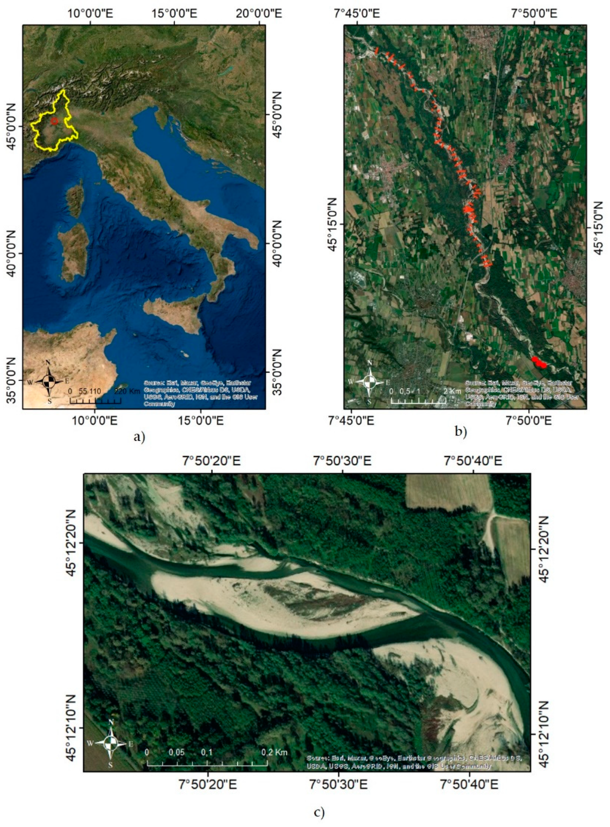
All the experiments showed in this paper have been based on one test site in Italy, chosen as representative and significative from a hydraulic and hydrological viewpoint. We tested and validated the methodology on the case study of a natural river of Northern Italy, the Orco River (Figure 1). This stream is a tributary of Po River, and it performs a sinuous-meandering planimetry interrupted by multithread reaches with islands and disconnected terraces. Orco River is one of the most dynamic watercourses in Italy, being its mean migration rate around 10 m/years, in particular, in the last 20 km upstream, the confluence with Po River. Its slope ranges between 0.0015 and 0.007, and sediment deposits contain coarse sand and pebbles, with a mean diameter of 7 cm. The Orco River shows almost pristine conditions in terms of geomorphology, hydraulic functioning, and vegetation ecology. In 1994 and 2000, flood events have had significant effects, with dramatic economic consequences. For these reasons, Orco River is subjected at important years-by-years monitoring plan. Moreover, it will be involved in major investments of river engineering, aiming to manage the basin sediment budget. All these activities require huge efforts for the extensive DTM generation. In the next section, all materials and methods considered in the measurement campaigns and the data processing activities are shown and described, specifically, highlighting the new Geomatics methodologies and tools employed and developed.
3. Acquisition Materials and Methods
In order to address the automatic recognition and refraction reduction in the water table directly on the dense point clouds, various operating procedures have been carried out. They are summarized as follows: (i) materialization of 110 georeferenced Ground Control Points (GCPs); (ii) evaluation of Control Points (CPs) through topographic acquisitions via GNSS receivers, associated with multiple bathymetric sections along the watercourse, with the aid of GNSS positioning in RTK and Network Real Time Kinematic (NRTK) mode; (iii) wherein the satellite visibility was really poor (e.g., close to the borders of the river or where the canopy covered most of the river bed), traditional topographic techniques, such as total stations, was applied; (iv) multiple UAV and UAV-RTK flights were carried out for the reconstruction of the three-dimensional models through the realization of some dense point clouds, using Agisoft Metashape Professional (AMP), a commercial Structure for Motion (SfM) software; (v) the previous step allowed us to obtain high definition spatial data, such as digital surface and digital terrain models (DSM and DTM, respectively) and orthophotos. However, the products at point (v) have not been relevant for this paper but will be used in future works. All topographic and photogrammetric acquisitions of steps (i)–(iv) will be detailed in the subsections below.
In order to obtain a suitable product for the case study, we provide a first-step identification of the water refraction error to correct the photogrammetric models. This rough model is based on a constant coefficient, which takes into account the different refraction indexes between air and water. As widely demonstrated by previous works in the same field [16,17,18,19], the primary approach derived from Snell’s law cannot represent a suitable and exhaustive bathymetry correction system. This drawback is due to the physical characteristics of the watercourse (i.e., nonplanarity of the free surface of the water, presence of waves, high depth, loss of water clearness, and the lack of light beam incidence in the optical path). The current literature is in fact rich of examples of algorithms based on constant refraction parameters [20,21], with many concerns on the limited validity of the approach, due to the spatial heterogeneity of watercourses.
3.1. Topographic Measurements for GCPs Acquisition and Bathymetric Sections
The aerial photogrammetric acquisition can be performed through two main approaches: (i) the so-called direct photogrammetry [22] and (ii) the use of GCPs. In the former process, the images are directly georeferenced from the information obtained through the accurate position of the center of the camera and the attitude angles. In the case (ii), it is mandatory to set some markers on the ground and to measure them through one or more geomatics techniques. Indeed, GCPs are points with well-known coordinates (estimated with GNSS instruments in static or RTK, to reach accuracies of few mm or cm, respectively), which are fundamentals to constrain the aerial photogrammetric model for the 3D reconstruction. These are points which the surveyor can precisely pinpoint, i.e., with a handful of known coordinates, it is possible to map large areas accurately. If some of them are settled in the riverbed, it is possible to compare the water depth measured with GNSS receivers with those estimated at the end of the photogrammetric processing. In the present work, we have followed the second approach, according to the procedure reported in [23]. In particular, after a planning phase, all the markers have been measured using three main techniques. In the zones where the Long-Term Evolution (LTE) connection was available, the GNSS NRTK positioning has been exploited considering the Virtual Reference Station (VRS) correction broadcasted by the SPIN3 GNSS network [24], as described in [25]. In the zones with excellent satellite visibility conditions, the single base GNSS RTK positioning has been considered, broadcasting the differential corrections, using a radio-modem or following a postprocessing approach [26]. In the zones with bad satellite visibility, we adopted a traditional topographic survey using a total station and a prism mounted on a pole.
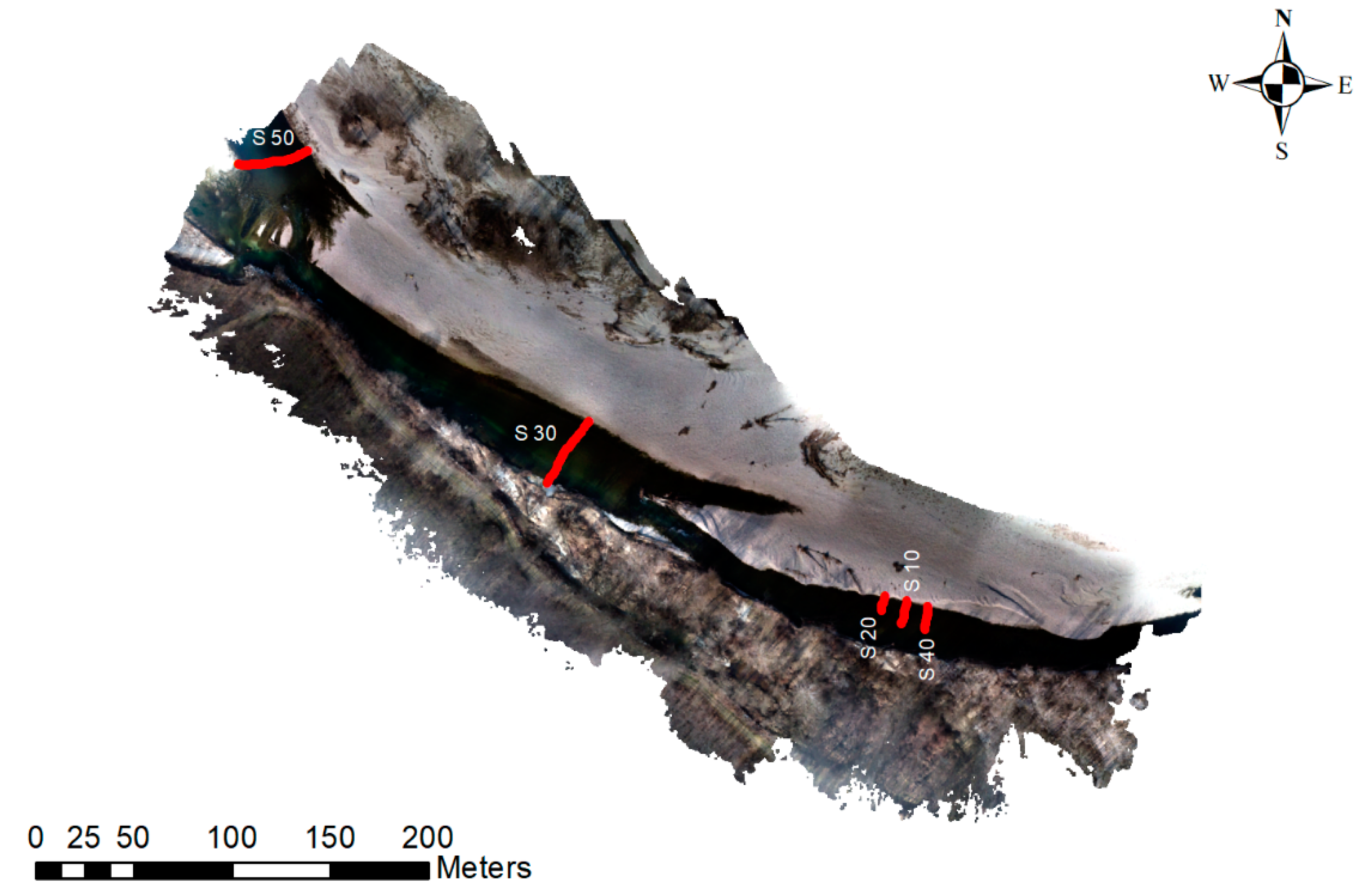
Five bathymetric sections, as reported in Figure 2, have been manually measured using the same approach of the GCPs. The water depth has been measured on 81 points forming the sections, using them as reference points for the correction of the water depth that will be described in Section 3. For all the points, the 3D accuracy obtained is smaller than 3.5 cm.
In all cases, the ellipsoidal heights have been converted in the orthometric ones considering the local model of geoid released by the Italian Geographic Military Institute (IGMI), using the GK2 grids and ConveRgo software. The local geoid model considered is ITALGEO 2005. It was computed at Politecnico di Milano and released by The Italian Geographic Military Institute (IGMI); this is the official tool that can be used to convert ellipsoidal heights into orthometric (or normal) ones. In this last release, the area covered by the estimate is 35° < latitude < 48°, 5° < longitude < 20° with a grid spacing of 2′ both in latitude and in longitude. The computation is based on remove–restore technique and fast collocation. The gravimetric geoid, integrated with GPS/levelling data, has an overall precision of around 3 cm over the entire Italian area.
3.2. Photogrammetric Data Acquisition and Processing
In order to obtain a source dataset appropriated to our purposes, we have postprocessed the photogrammetric data. The Orco River is morphologically organized in many particular environmental units, which require careful flight planning for several daily surveys. Therefore, the aerial images have been acquired during four different survey campaigns using UAV flights in RTK configurations, obtaining thousands of nadir and oblique images [27]. The choice of a manual flight plan has allowed high levels of safety for operators, and the standard criteria of terrain resolution and accuracy of the photogrammetric products have been guaranteed [28].
Three commercial UAVs have been used:
- DJI Phantom 4, with an FC6310 camera, 20 MP CMOS sensor, and a focal length of 8.8 mm.
- DJI Phantom 4 RTK, with an FC6310 camera, 20 MP CMOS sensor, and a focal length of 8.8 mm.
- DJI Mavic PRO, with an L1D-20c Hasselblad camera, 20 MP 1 sensor, and a focal length of 10.26 mm.
Data regarding the images acquired concerning the flights carried out during the relevant survey campaigns are summarized in Table 1.
To obtain the needed photogrammetric products, 6152 frames have been processed, using GCPs to georeferencing the subsequent point clouds, and CPs to evaluate them. The methodology for the correct identification and correction of the refraction is reported in Section 3.
To generate many digital models suitable for the automatic classification analysis, a specific standard criterion for the UAV frame processing has been used. To this aim, all images have been imported in Agisoft Metashape Professional (AMP), a commercial Structure for Motion (SfM) software, which is common in photogrammetric block processing, and installed on Intel(R) Core (™) i7-4770 CPU operative system (3.40 GHz) workstation, with 32.0 GB RAM.
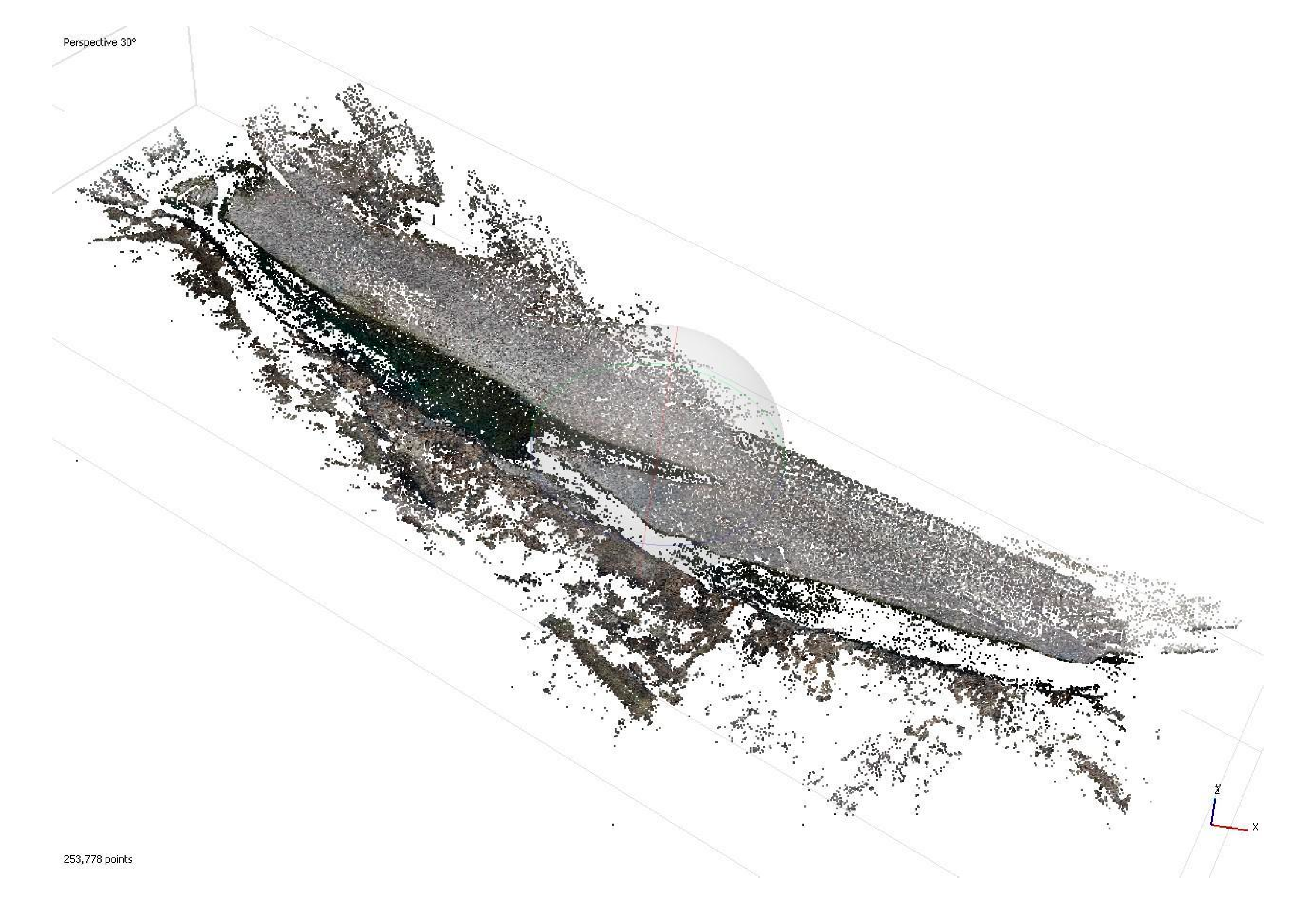
The procedure has required a subdivision into four different projects, one for each survey campaign. Each project has been further differentiated in chunks, based on the performed flights, taking into account the average flight altitudes and the use of nadiral and oblique images to improve the resolution of the final products. Then, any frame of each chunk was aligned, to identify a first scattered point cloud (named “sparse points cloud”) from the automatic recognition of the characteristics contained in every pixel between 2 and more superimposed frames. Such homologous points (called tie points) can be obtained employing three different levels of accuracy: Low, Medium, and High, respectively, with the increasing number of tie points. To generate clouds as accurate and precise as possible, the “High” level has been set for all the chunks processed. Figure 3 shows a scattered point cloud example, as obtained using AMP.
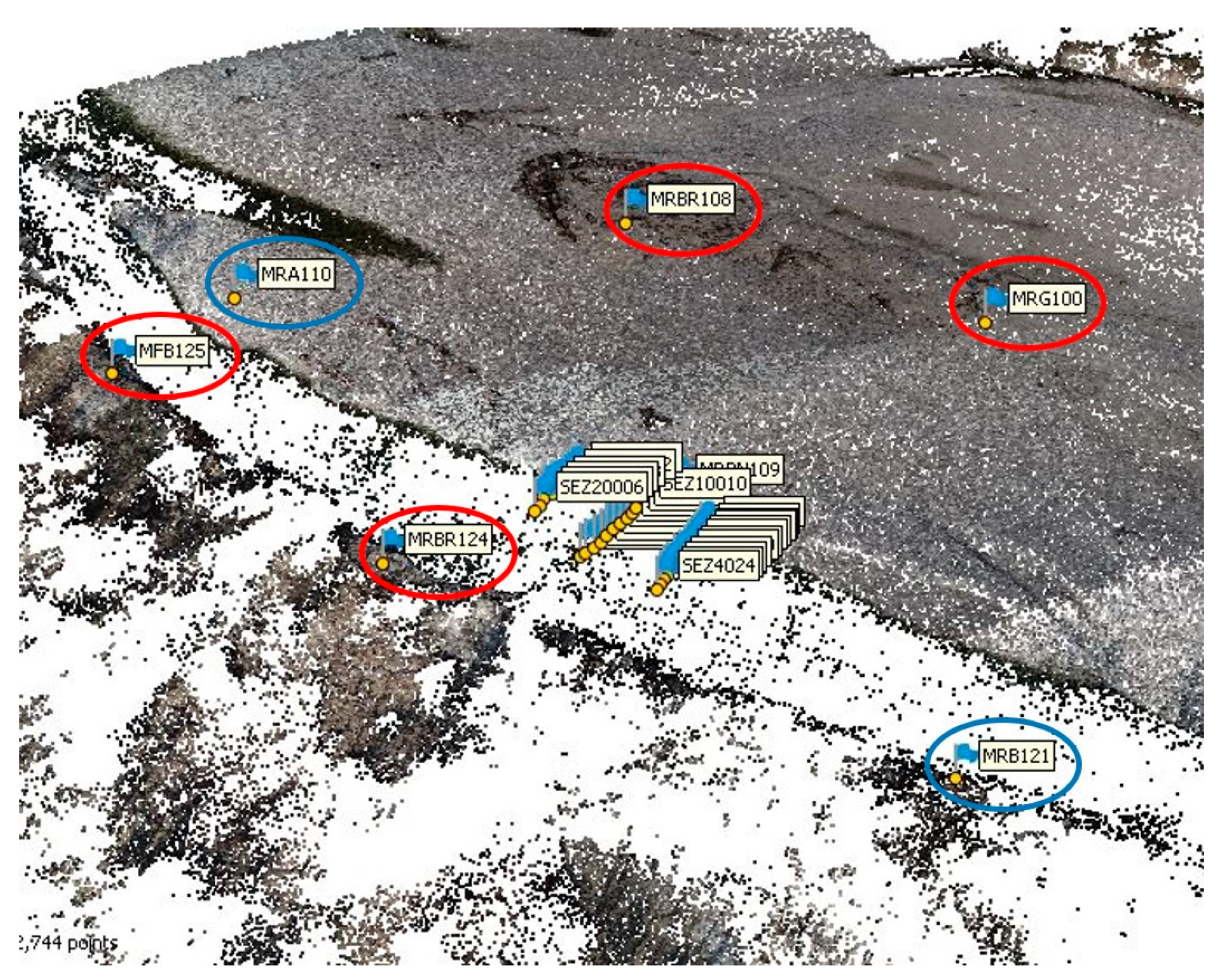
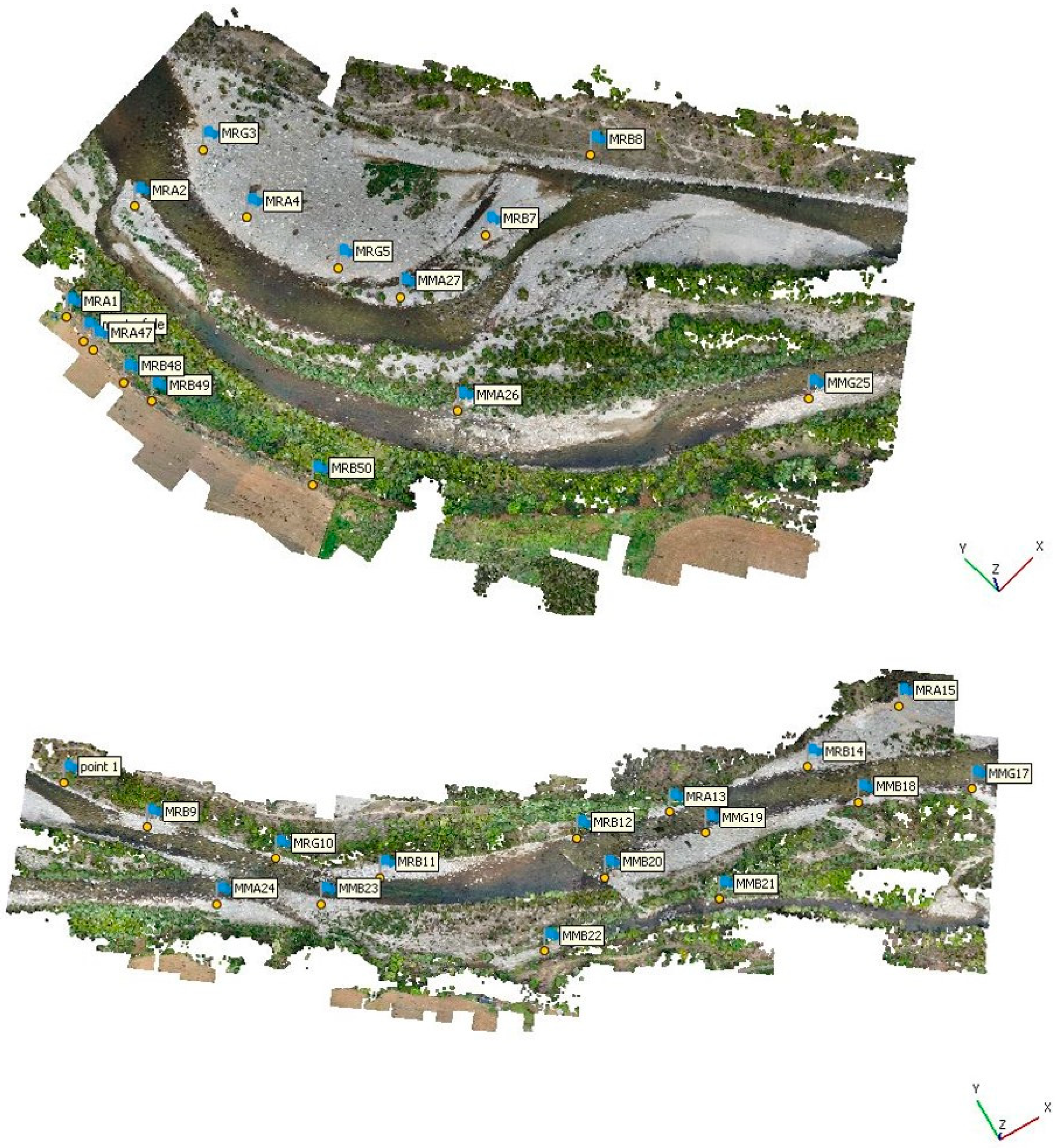
Since the scattered clouds are thus obtained without a reference datum, the text files (.txt format) containing the coordinates of the markers for UAV-derived images (GCPs and CPs, see also Figure 4 have been imported into AMP. We recall that the frames taken through UAV-RTK configuration are already georeferenced, and this last operational step is not necessary, but it is suitable in order to optimize the camera interior parameters estimation and to improve the generation of the photogrammetric block.
The GCPs and CPs markers have been identified using their shape and spatial distribution in relation to the area extent enclosed in the scattered point cloud. Furthermore, the GCPs have been collimated in all the frames in which they have been found, taking care to obtain a residual error less than 3 cm. The CPs markers have been used as validation on the precision achieved in the georeferencing phase. Table 2 and Table 3 show the residual values obtained for each computed three-dimensional model.
Subsequently, all dense point clouds have been automatically processed using the appropriate tool present in AMP. The dense point clouds constitute our final processing data, and the dataset for the following automatic classification analysis and refraction correction methods will be performed. To this aim, similarly to the alignment phase, a highly detailed level has been set. Dense point clouds with high detail scale (1 point every 4 cm) have been computed, suitable for large-scale investigations (1:200). Table 4 reports the characteristics of the generated dense point clouds, expressed in terms of total number points, processing time, and the respective average densities.
We remark that the generated dense point clouds present a moderate level of noise, due to the presence of high and medium-sized vegetation in the survey areas, as well as the boundary-effects in the photogrammetric block. To reduce the impact of this problem on the overall accuracy of the individual three-dimensional models, these clouds have been manually cleaned; the manual cleaning has been made to avoid all the failure points, such as natural clouds or different anthropic issues.
4. Refraction Correction Processing
Using the photogrammetric product obtained (i.e., high details dense point clouds), the main goal for the authors has been concerned with the accuracy and precision evaluation of the water points present in the dense point clouds: as it is previously described, the estimated points in the riverbed are affected by many errors, such as the refraction law and the photogrammetric distortions. Thus, the first step of this work is to demonstrate the reliability of the innovative methodology for the reduction in the refraction error on photogrammetric data in fluvial environments, as we developed here. Two different methods and approaches have been followed: (i) a simplified approach based on Snell’s law and (ii) a new methodology based on an innovative polynomial correction based on the physical and photogrammetric characteristics of the investigated object.
4.1. Bathymetric Reconstruction Using Atmospheric Snell’s Law Index
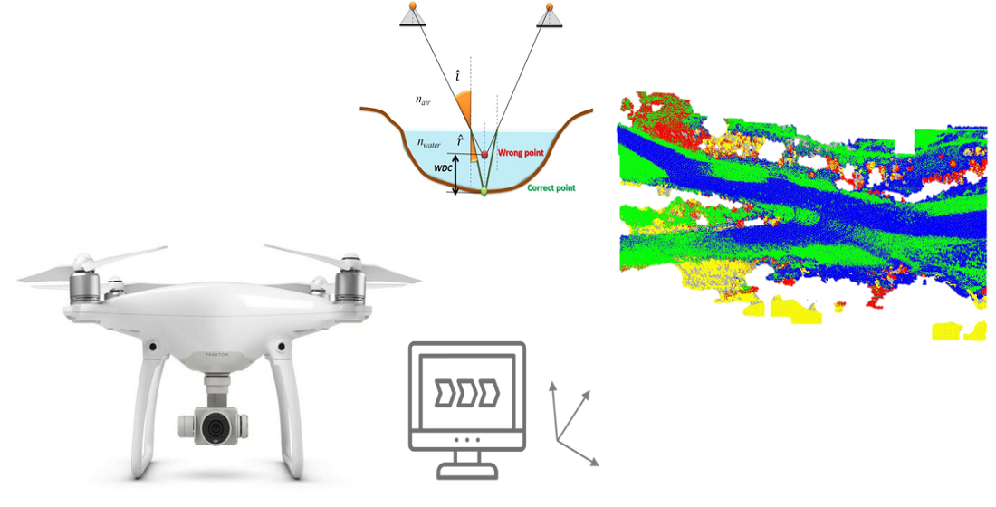
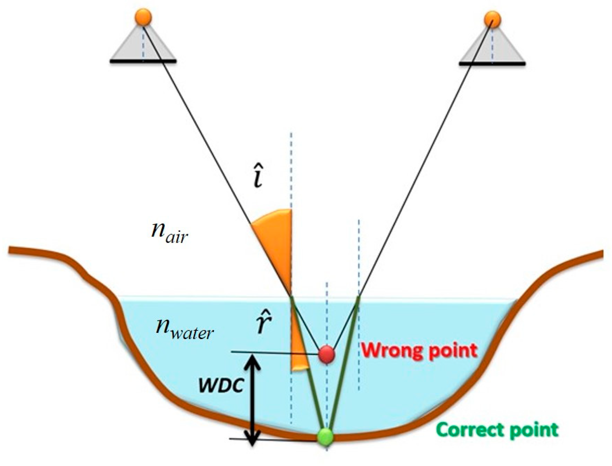
The approach is based on the Snell’s law index only, which describes the refraction at the water–air interface due to the change of refractive index. Thus, the river bathymetry can be reconstructed using the homologous ray’s correction from the photogrammetric information, to resolve the underestimation of water depth due to refraction, through Snell’s law approach (Figure 5).
The analysis has been conducted only on the photogrammetry dense point clouds, by selecting every point related to the water table (named “wrong points”). The correction parameter called Water Depth Correction (WDC) have been applied only on these points, following the Snell’s law index:
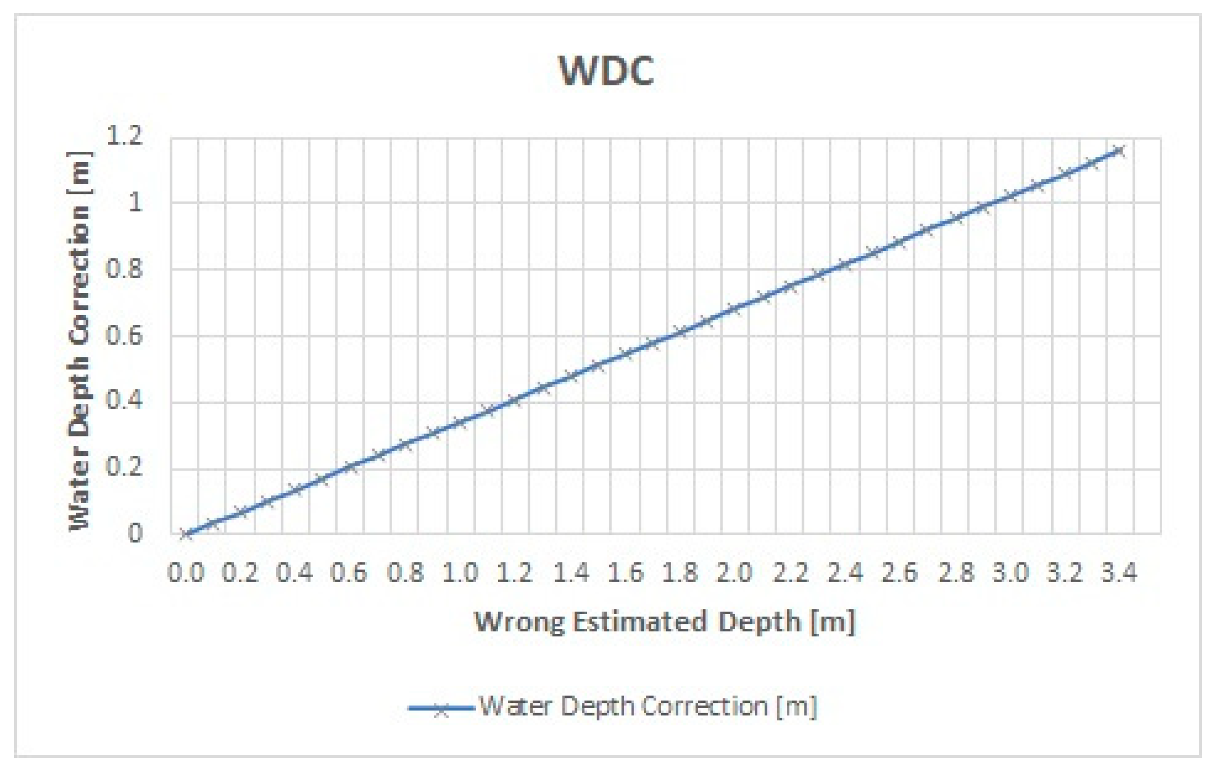
In a standard photogrammetric case (i.e., points with the same distance between image projection centers and about 70% of images overlap), WDC is linearly related to the wrong estimated depth and, in a first approximation, the correction factor is about 34%, as shown in Figure 6.
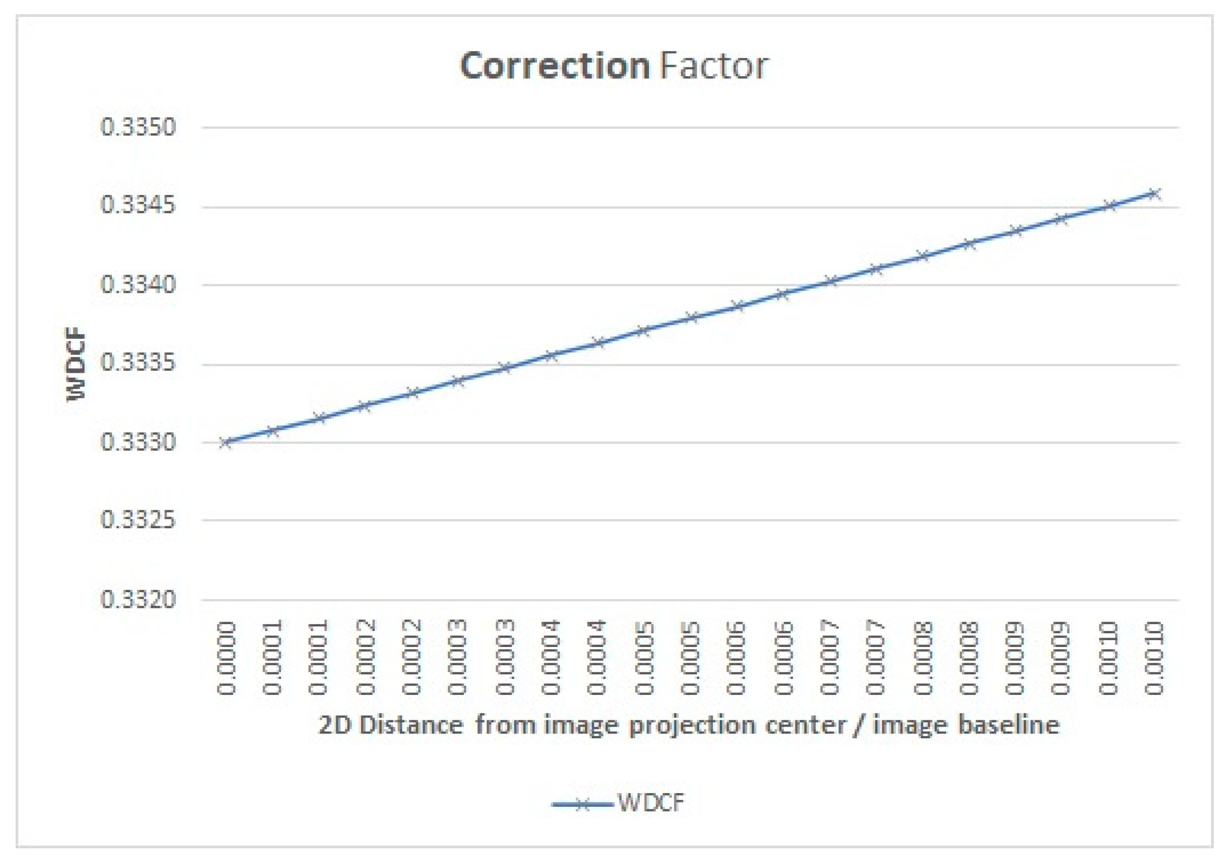
Approximately, the WDC depends on the 2D distance between the wrong point and image projection centers. In a general way, the WDC variation can be defined as a function of the ratio between this distance and the image baseline (Figure 7).
In Figure 7, the estimated water depths have been corrected by applying a constant factor of 1.335. However, this process can be used only in the presence of very shallow clean water depths and a planar water table without waves, where the riverbed is well visible from the acquired photogrammetric images.
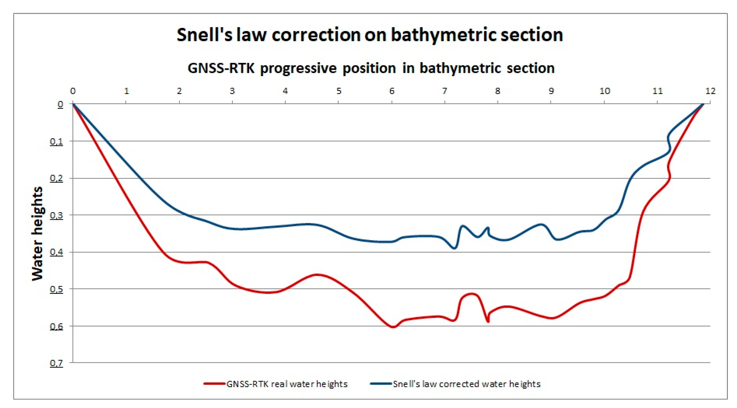
Due to the limitations, as mentioned earlier, the case study presents variable conditions in terms of depth and clarity of the water column, high flows, and the presence of rapids. The application of the Snell’s law correction index did not bring acceptable results in terms of precision. In Figure 8, it is evident that the application of this correction factor led to errors of order 10–15 cm, not suitable for large-scale studies. For this reason, a second approach has been improved.
4.2. Bathymetric Reconstruction Using Linear Regression
To increase the performance of the bathymetric corrections, we calibrated a linear model on the topographic points in the river. Those points have been selected where the water depth is known with good precision, considering five cross-sections of the river, with different conditions of illumination, river depth, and riverbed. We used them as our testing population, to calibrate the system with a linear model and to extrapolate the same water depth from the points of the digital model.
For any point, we calculated the water depth, excluding the ones with depth less than 0.1 m, where almost no correction was necessary. Then, we coupled every topographic point with its closest point extracted in the digital model, calculating the water depth using the same water level as the reference. The topographic points have been measured through GNSS-RTK technique, obtaining five sections. We developed a linear relationship between the water depth obtained from the topographic points (WT) and the wrong water depth obtained from the digital model (WD), such as:
The intercept and the angular coefficient were easily calculated using a least-square linear regression between the topographic and the digital model water depths.
This basic model was improved by taking into account the contribution of the radiometric information provided by the images acquired from drone flights. To this aim, we assumed that the watercolor in a drone-acquired image is affected by illumination, water surface disturbances, riverbed material, and water depth. All these factors influence the errors of the digital model. Since the color of every photogrammetric point in the acquired image is known, we calibrated a multiple regression model that takes into account both the water depth obtained from the digital model and the RGB (Red, Green and Blue) colors of the image, as predictors for the topographic water depth:
where R-G-B are the 16-bit color values in the image. The regression model was performed with MATLAB, using the fitlm function, which calculates the coefficients and the statistics of the regression.
We build a sample of 72 manually measured points by mixing all the points from the five sections. To evaluate the performance of the regressions, we used about 85% of points, randomly selected, as a calibration sample, and we tested the performance of the prediction on the remaining 15%. For every testing point, the error was calculated as the difference between the water depth prediction (WPRED) and the true one (WT), as described in the following equation:
The mean error and the root mean squared error were also calculated. To obtain a robust evaluation of the regression model performance, we repeated calibration and test operation 1000 times, by shuffling the elements of the calibration and the test sample each time randomly in the MATLAB code. The results presented in Section 5.1 are the mean statistics of the performance over those 1000 runs.
5. Machine Learning for Automatic Classification of Dense Point Clouds
As shown in the previous sections, it is possible to perform an automatic bathymetric correction of many sections. Still, first, it is crucial to determine and characterize the dimensions of the river planimetry accurately. A key point is to detect the borders of the watercourse to select the points that require a correction. If large portions of the fluvial corridor are under investigation, this step cannot be addressed manually, and automatic characterization becomes mandatory. To achieve this goal, we have developed an algorithm to recognize and classify the water table and land areas directly on the dense point clouds. Accordingly, we developed a novel procedure using ad hoc machine learning (ML) technique, which can identify four main classes:
- Water, identified as the area displayed in the dense point cloud that is circumscribed by wet contours (riverbanks), either natural or artificial. Its correct classification is the first fundamental step of the procedure.
- Gravel bars, identified as all the planforms composed by sand-gravel sediments with variable grain size—from coarse sand to centimeter pebbles, up to decimetric boulders—transported by the river during high flows. The gravel bars are sited both in large bodies (point bars) in the inner banks of meanders and the main body of the watercourse, as well as in central river bars (elongated and narrow) occurring in the middle of the river.
- Vegetation, defined as the cover plant that is present along the wooded terraces on both sides of the investigated reaches (typically mature vegetation) or associated with sparse vegetation that is present on gravel bars (typically bushes). Any large log detected in the riverbed that is mobilized during high energy events was also identified.
- Ground/Soil, including undergrowth areas, grassy meadows, agricultural fields, roads, and paths, possibly present in the analyzed regions.
The procedure involved a series of operations on the photogrammetric datasets (i.e., dense point clouds), followed by the editing of an automatic classification code in Python language and using the Random Forest algorithm. All the operating steps composing the workflow are listed and described in the following sections.
5.1. Dense Point Clouds Management: Export and Cleaning
To proceed with the dense point clouds classification, we previously considered their goodness in terms of noise points, which could affect the quality of the classification. With this in mind, the dense point clouds once obtained have been exported to the more manageable text data format on which all subsequent procedures have been performed. During the export phase, some fundamental parameters were set, such as the desired coordinate system and decimal precision.
The exported dense point clouds have been imported into the free and open-source Cloud Compare (CC) software to complete a first review and cleaning phase. Specifically, an algorithm implemented in CC for the analysis and noise reduction, called SOR-Statistical Outlier Removal, has been adopted, and the main scattered points were eliminated. Furthermore, any other scattered points not identified by the filter have been manually eliminated, focusing on any remaining scattered points.
5.2. Annotation and Geometric Features Computation
The next step has required the definition of the input parameters for the ML training phase suitable for classification; to realize it, some training and testing dense point clouds have been chosen. The definition of the input parameters for the ML training phase and the selection of the dense point clouds for these analyses was subsequently improved. The point clouds of day 16 April 2019—regarding flights 1 and 4—have been selected as the training dataset, while the dense point cloud obtained on the same day in flights 2 and 3 have been chosen to test the performance of the selected classification algorithm. Figure 9 shows the training-testing dense point clouds dataset.
Many geometric features available on CC were calculated: the most indicative one is based on eigenvalues, which are related to the shape and density of the analyzed dense point cloud. The eigenvalue-based features have been obtained by setting a single parameter, the so-called Local Neighborhood Radius, which represents the radius within which the algorithm selects the points of interest and the transformation parameters (i.e., eigenvalues and eigenvectors).
The eigenvalues represent the scalar values in the vectors transformation (eigenvectors) of an original matrix dataset (raw data present in a dataset), leading it to a reduction in the dimensionality:
where M is the original sparse matrix (dataset), o is the transformation vector (eigenvector), and n is the scalar value (eigenvalue).
Using these particular values, we were able to calculate the following geometric features, based on eigenvalues L1, L2, and L3 about the X, Y, and Z coordinates of the original dataset:
- Eigenvalues Sum, that is the sum of the three eigenvalues corresponding to the respective spatial coordinates of the reference system.
- PCA1 (Principal Component Analysis), the dimensionality reduction on L1 eigenvalue.
- PCA2 (Principal Component Analysis), the dimensionality reduction on L2 eigenvalue.
- Planarity, the planoaltimetric envelope of the analyzed points in the dataset.
- Linearity, a feature based on the shape of the cloud itself.
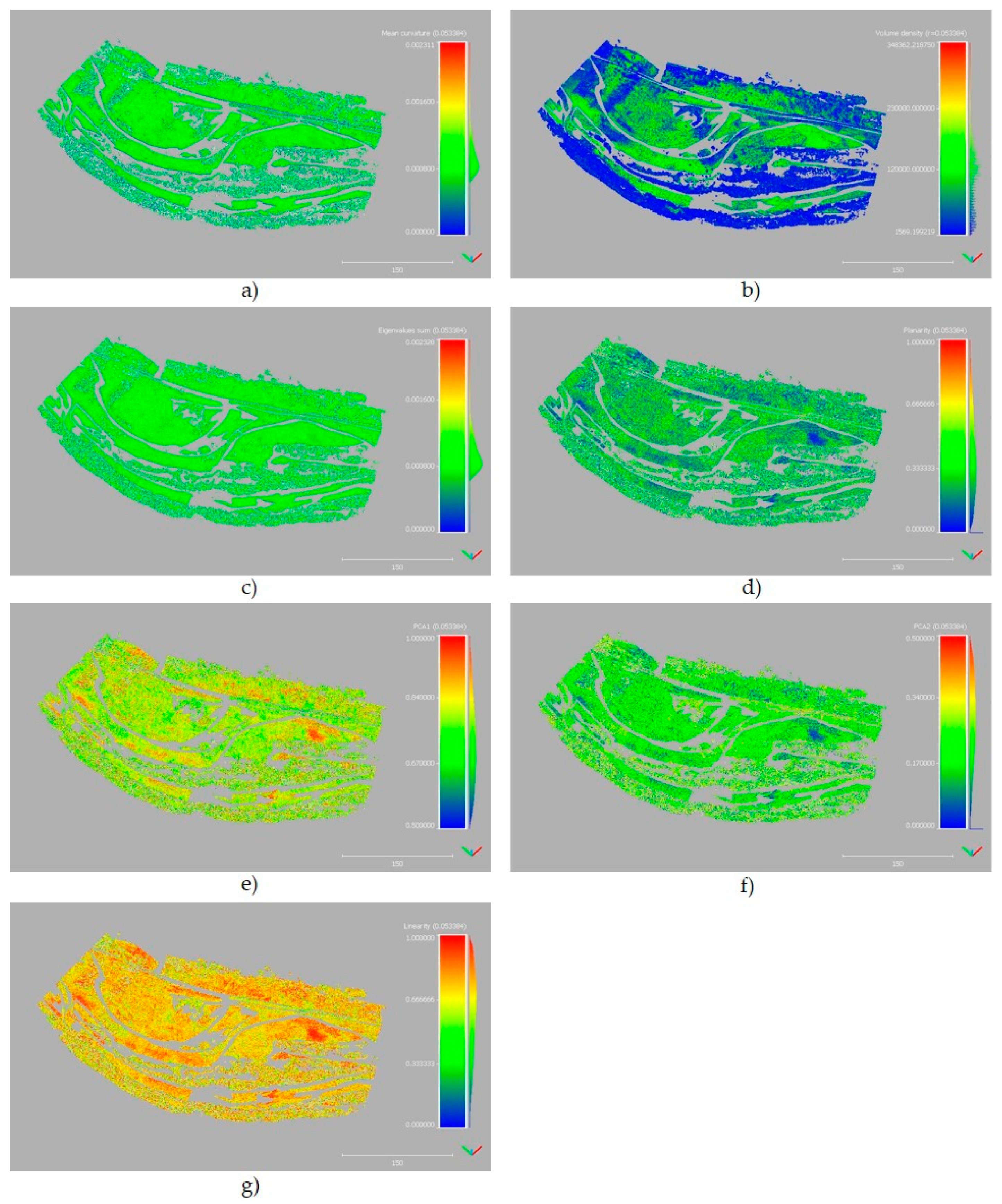
Two other geometric parameters have been computed, using the same calculation tool: Mean Curvature, and Volume Density. These parameters refer more specifically to the shape and density of the points with respect to a specific volume defined by the input value of the Local Neighborhood Radius. Geometric features and shape-related issues are shown in Figure 10.
The aforementioned geometric features have been selected to obtain a more valid and complete training dataset as independent as possible by spatial correlations. Moreover, the interaction between the computed geometric and shape-related features has allowed defining a training dataset for automatic classification using the ML algorithm described in Section 5.3. Further geometric and nongeometric parameters will be researched and implemented in forthcoming works aiming to increase the spatial validity of the ML algorithm, as well as the accuracy during the training phase.
The calculation of these parameters has been performed on both the training and testing phases to generate a statistical relationship between them. The standard procedures stop here: to develop a complete neural network capable of carrying out an accurate classification, it was necessary to associate the characteristics mentioned above to the desired classes (i.e., Water, Gravel bars, Vegetation, and Ground/Soil), creating a unique scalar field called Class. The operation has been carried out on the training dataset only, by assigning these classes through manual annotation, i.e., each zone has been associated to a numerical code (11, 22, 33, and 44 corresponding to blue, green, yellow, and red, respectively, as shown in Figure 11), necessary to limit the errors and the processing time of the ML algorithm in Python, as described later. The manual annotation of the classes was based on the individual interpretation by the operator, distinguishing wet areas from other classes (Vegetation, Gravel bars, and Ground/Soils) by means of the RGB bands computed on the dense point cloud. To improve the performance of the algorithm, for each Class, the same number of points has been assigned to avoid that the classifier algorithm hierarchically gives different weights to them, as described in [29].
The training and testing dense point clouds, properly implemented, have been finally exported to text files taking care to indicate the value of the decimals as accurately as possible, at the same time considering their weight in terms of space and visual memory on own workstation.
5.3. ML Algorithm: Random Forest Classifier in Python Languages
We designed a special ML algorithm using the Python language, by exploiting appropriate libraries already available online (i.e., [30,31,32,33,34]). The automatic classification algorithm developed in this work is based on the Random Forest [35,36], present in a specific Python library called Scikit-learn, which is composed by a series of “n” decision trees that exchange information with each other to achieve a correct classification and minimize overfitting errors.
Before applying the algorithm, some preliminary steps were necessary to analyze and correct the training dataset, exploiting different libraries already available, such as NumPy, Matplotlib, and Pandas. In particular, the preliminary operations are summarized as follows:
- Cleaning of the training dataset, identification of any missing point (non-numeric) (NaN) data, through the use of dropna() function.
Training_dataset = pd.read_csv(“Source file”, sep = ‘,’, error_bad_lines = False, low_memory = False)
Cleaned_dataset = Training_dataset.dropna().
Cleaned_dataset = Training_dataset.dropna().
- Analysis of the training dataset dimensionality, in order to check if each of the 4 classes has the same order of magnitude in terms of the number of points, using the value_count() function in a targeted columns useful into classification.
11.0 490577
22.0 488373
33.0 454210
44.0 363000
Name: Classe, dtype: int64.
22.0 488373
33.0 454210
44.0 363000
Name: Classe, dtype: int64.
- Subdivision of the dataset into two main parts: classification parameters (labels) and desired classes, using the drop () function
X_train = Cleaned_dataset.drop(columns = […],axis = ’columns’)
Y_train = Cleaned_dataset[…].
Y_train = Cleaned_dataset[…].
- Normalization and fitting of the classification parameters (labels) of the training dataset. In the Scikit-learn library (Preprocessing module: Label Encoder), some transformation and normalization functions (fit_transform) of the values are implemented, in order to make them more significant during the subsequent classification phases. Hereinafter, an example regarding PCA1 values is shown.
le_pca1 = LabelEncoder()
X_train[“pca1_n”] = le_pca1.fit_transform(X_train[“PCA1 (…)”]).
X_train[“pca1_n”] = le_pca1.fit_transform(X_train[“PCA1 (…)”]).
- Implementation of the Random Forest algorithm. The Scikit-learn ensemble library contains many different ML algorithms, including the one chosen by the authors. The Random Forest Classifier has various setting parameters, useful for adapting to any different request, as described in the official website [35]. In the specific case addressed, several tests have been carried out, identifying the ideal configuration when the number of estimators is defined as 100. The configuration has been allowed to obtain a good compromise between the classification’s precision and the processing time.
Model = RandomForestClassifier(n_estimators = 100).
- Training phase. This step has been made using the fit() function, specifying the Random Forest model and the dataset to be used, i.e., the aforementioned dense point cloud previously optimized.
Training_model = model.fit(X_train, Y_train).
- Testing phase. The testing phase has been carried out by merely recalling the trained model, indicating the dataset on which to test, using the predict() function. Repeat the (12) and (13) phase aforementioned, using only the transform() function to normalize the Labels data.
Test_dataset = pd.read_csv(“Source file”, sep = ‘,’, error_bad_lines = False, low_memory = False)
…
Y_predict = model.predict(X_testing).
…
Y_predict = model.predict(X_testing).
- Point cloud export. Finally, the dense point cloud classified in text format has been exported to be able to see it in a point cloud management software.
np.savetxt(“Output name.txt”,my_data_1,delimiter = ’,’,header = ’…’).
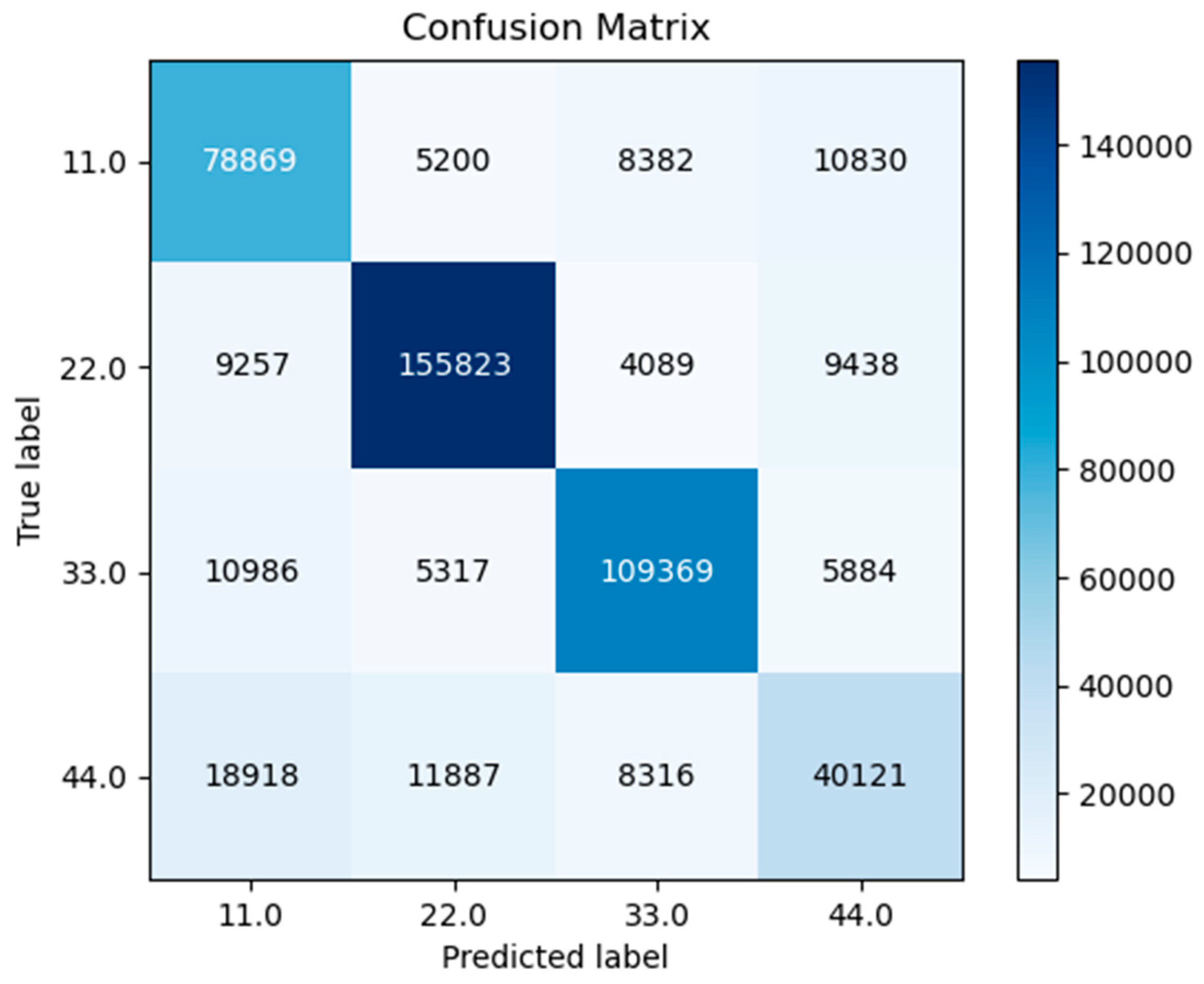
- Evaluation of accuracy parameters: for this step, the train_test_split function and the Sklearn.metrics library [37] have been widely used. To identify the quality of the classification, the following parameters have been calculated: Accuracy Score, Precision, Recall, and F1-score. Most of them are based on the relationships between the True Positive (Tp), False Positive (Fp), True Negative (Tn), and False Negative (Fn) values obtained from the Confusion Matrix.
6. Results
6.1. Bathymetric Corrections Using Linear Regression
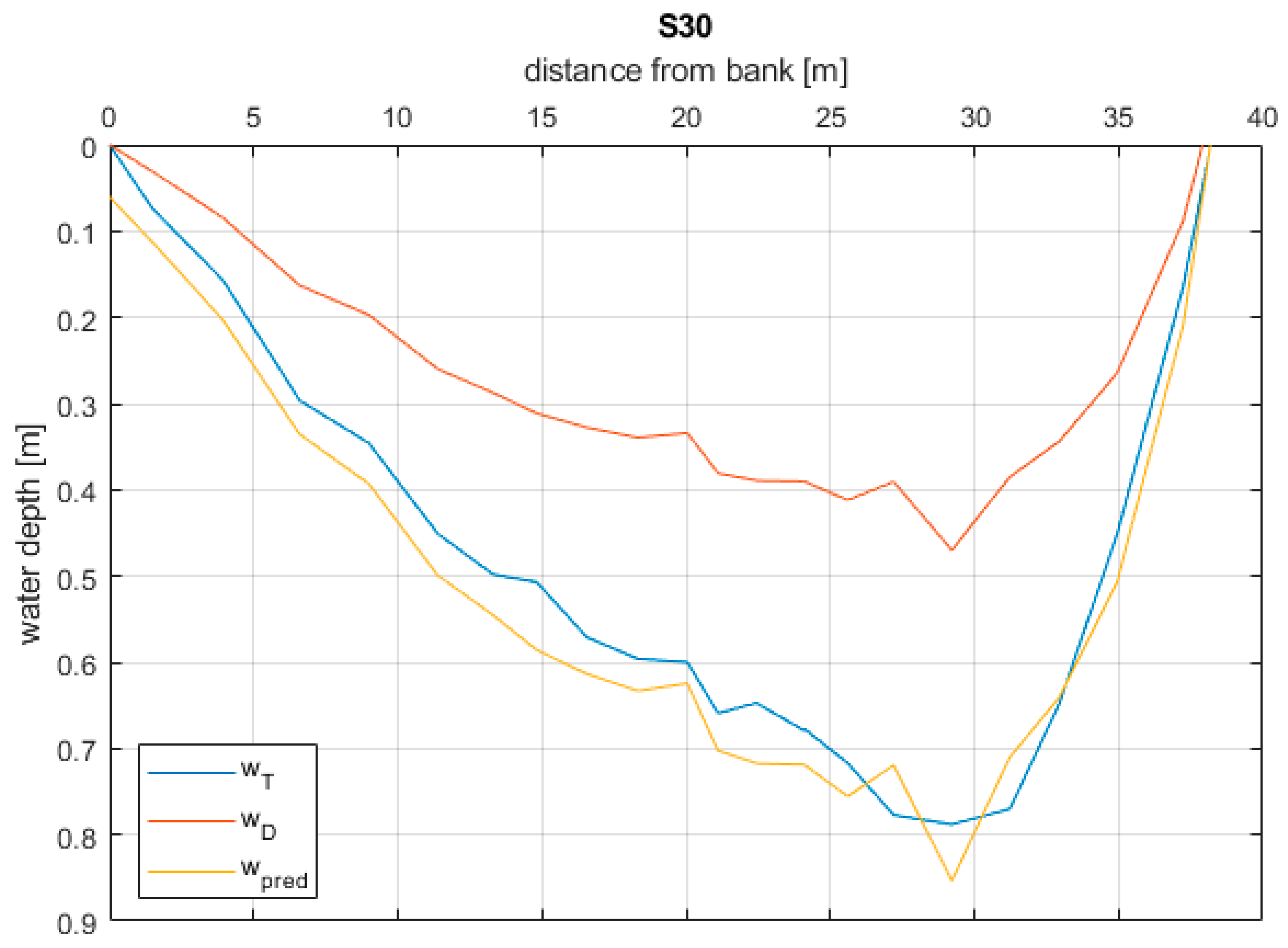
In this section, the performances of the multivariate linear regression described in Section 3.2 are evaluated. As written above, the calibration and test operations were repeated 1000 times with randomly chosen subsamples. The estimated regression coefficients are calculated as the mean over the 1000 iterations, and the performances have been assessed reporting the absolute mean and the root mean square errors. The absolute mean error over the whole set is 6.2 cm, and the RMSE is 7.6 cm. These values can be considered acceptable since they are of the same order of magnitude as the median size of the granulometric distribution of the riverbed sediment for the Orco river in the study area (namely, the D50 diameter), that is 7 cm. Therefore, the obtained average error in the depth predictions has same size of the median riverbed material. A comparison example between the water depth reconstruction obtained with the proposed method and the topographic water depth measured with GNSS-RTK technique is shown in Figure 12, where the section S30 is reported.
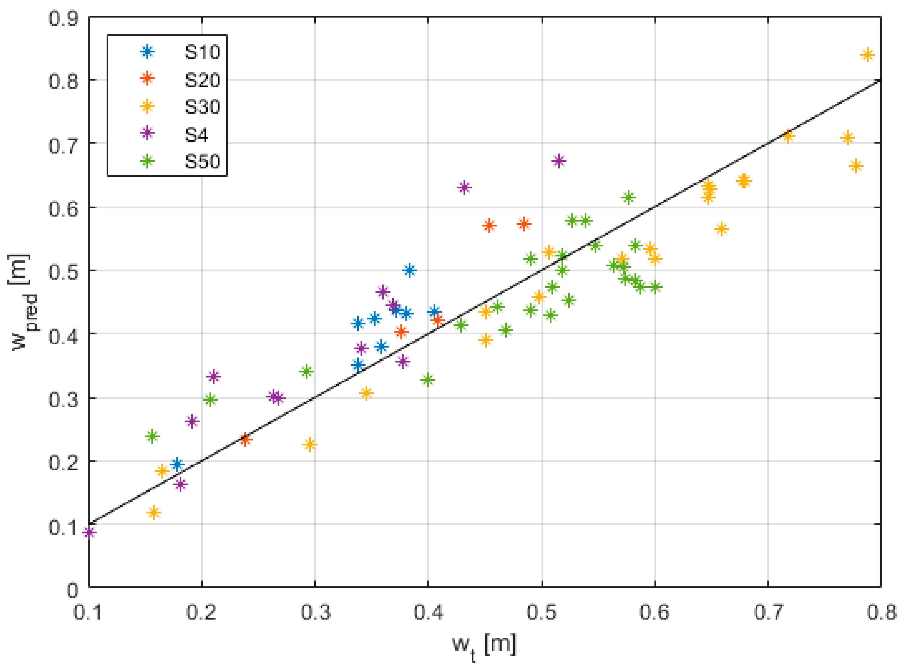
The goodness of the obtained results can be observed in Figure 13, reporting a scatter plot of measured versus model-predicted, for all the cross-sections. We remind that the same regression was applied blindly to the whole dataset.
We can notice a generally good agreement between predicted and measured depths. It is also evident that the error is not constant over the different sections. Therefore, the method can be improved by taking into account other fluvial environmental characteristics, such as riverbed material and water surface inclination, coupled with the photogrammetric processing variables, such as distortion parameters (Ω, Φ, and Κ) and the camera orientation (roll, pitch, and heading).
6.2. Machine Learning Results: Dense Point Clouds Automatic Classification
By implementing a Random Forest-based ML algorithm, we estimated the refraction reduction in a riverbed from dense point clouds obtained through the photogrammetric process. Additionally, a dedicated application of a classifier algorithm using the Python language has been developed. The integration between the two techniques mentioned above has allowed the authors to obtain an automatic classification of the water table. Specifically, the photogrammetric processing led us to the generation of 7 dense point clouds distributed in 4 survey campaigns, with 6800 images acquired in 21 UAV flights overall; these data show a detailed investigation scale, with an average density of about 26 points/dm2.
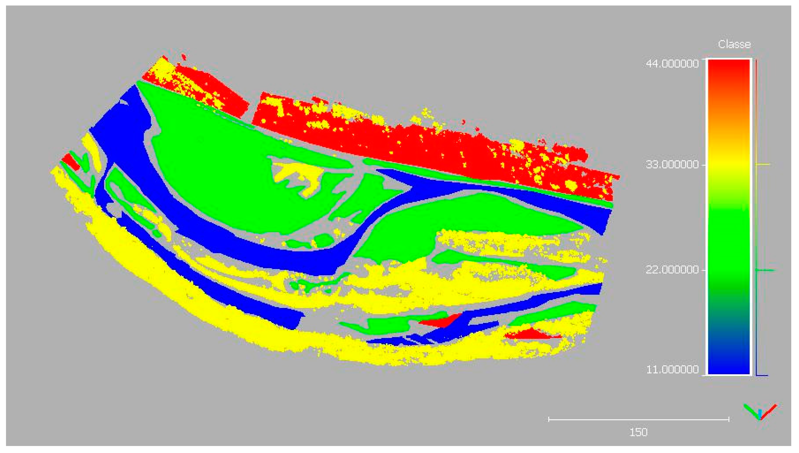
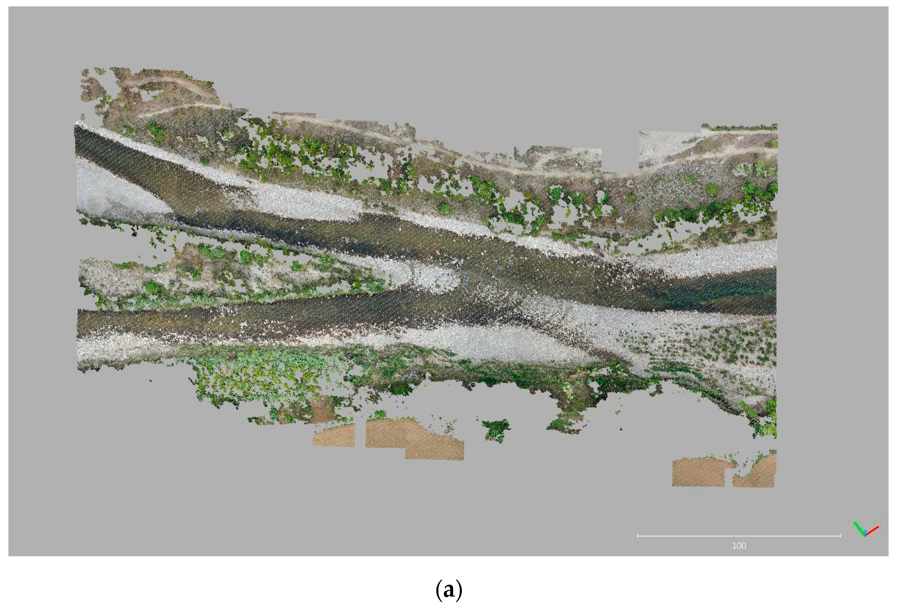
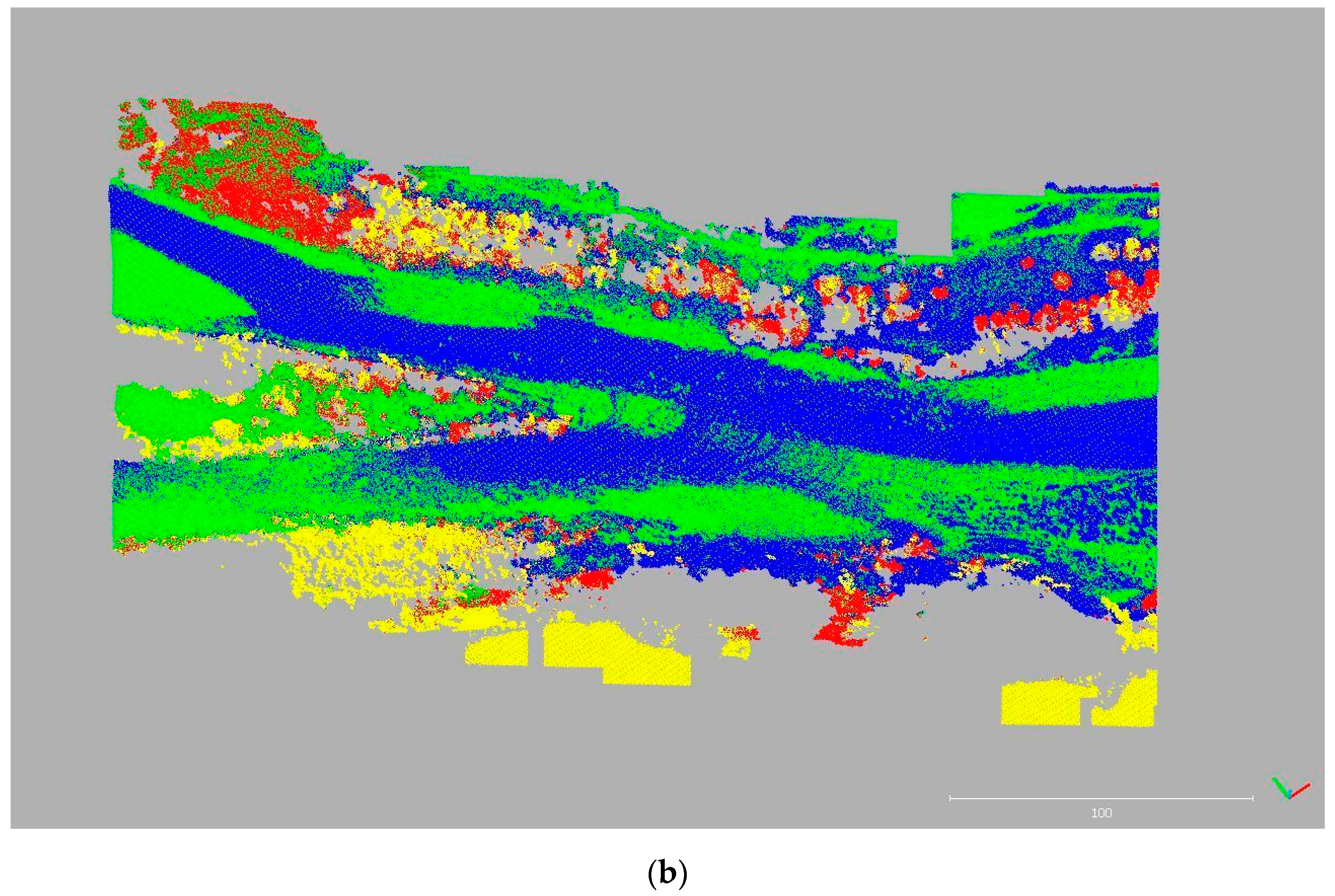
By writing the appropriate ML code in Python for the automatic classification, the accuracy parameters (i.e., accuracy score, recall, precision, F1-score, and the confusion matrix), summarized in Table 5 and Figure 14, have been obtained on the testing cloud to the training dataset. It has been appropriately implemented in four different classes (Water [Class 11], Gravel bars [Class 22], Vegetation [Class 33], and Ground/Soil [Class 44]) as it is possible to see in Figure 15.
Comparing Figure 15a,b, it is possible to conclude that the automatic classification methodology developed in this work has high validity in case of ideal radiometric radiation and spatial distribution of points. It is mainly due both to the nature of the RGB bands obtained from the photogrammetric process and the geometric parameters used during the training phase. If these ideal conditions are not reached, the quality of results becomes worse; so, it is possible to conclude that this preliminary step is only an earlier phase in automatic classification methodology, and it will be developed in forthcoming works.
7. Discussion
The bathymetry reconstruction using UAV is not a novel approach, i.e., previous studies using optical imagery-based bathymetry assessed the bathymetric data against other depth data, rather than bathymetry converted to elevation data (e.g., [21,38,39,40,41]). The decrease in accuracy when comparing underwater elevations to RTK-GNSS-measured elevations is likely due to imprecision in the water surface model used to convert the depth values to elevation values.
The methodology developed in this research activity for the identification of the river free surface and bathymetry through image detection from UAV, and the refraction correction due to the light radiation, has allowed us to assess the relation between photogrammetric detection and fluvial hydromorphology.
The quality and resolution of the obtained data is one order of magnitude higher than those obtained in the past considering LiDAR data [42,43,44] and river channel bathymetry obtained with photogrammetry [45,46,47].
Both the horizontal and vertical errors have been evaluated in this study; these two types of error are inextricably linked when ground elevations vary significantly with spatial position. We here considered a river with a maximum water depth of about 80 cm, obtaining good prediction on the identification of the benthic substrate, but these preliminary results do not guarantee that the same accuracy is reproducible with a deeper current (e.g., up to 1.5 m). We aim to investigate this aspect in the future works.
However, thanks to an ad hoc ML code, the present results suggest a substantial validity of the developed methodology, albeit with the limitations due to the classic radiometric parameters (RGB bands). This approach has been extensively employed in environmental remote sensing research [37,48]. The present ML technique, which is designed for the identification of wet areas in the fluvial environment and is combined with refraction correction applied to dense point clouds, provides a novel procedure with a great potential for future developments. In addition, it opens to new perspectives on the morphometric characterization, since it allows some morphometric characteristics to be readily assessed (e.g., river width, braiding index, and bank detection), with further advances in the analysis of single and multithread channels. We finally remind that the present approach is affected by the well-known limitations of any photogrammetric acquisition (i.e., distortion parameters Ω, Φ, and Κ and the position of the image centers).
8. Conclusions
The bathymetric reconstruction using point clouds obtained from UAV photogrammetry is an unsolved problem due to the difficulties to define the bed elevation of the wet surface. It also happens if Lidar instruments are considered as well. The only way to obtain a sufficient 3D reconstruction of the riverbed is to perform surveys during low flow hydrological conditions, while wet points are then detected with traditional methods. Thus, it is crucial to identify a new methodology to overcome these limits, to speed up the procedures of riverbed reconstructions, useful for engineers and decision-makers.
In this paper, a methodology useful for the free surface table and bathymetry identification in a river environment has been presented, with an error due to the refraction of light radiation obtained in the photogrammetric data processing phase. The study carried out the refraction reduction starting from classic in situ surveys and the processing of photogrammetric data obtained through UAV technologies. Four different measurement campaigns have been considered, performing 21 UAV flights, where 6800 images have been collected to have an average density of the final 3D model of about 26 points/dm2. These data have been used for the automatic 3D reconstruction using dedicated photogrammetric software, considering 76 GCPs collected with GNSS instruments in RTK mode for the georeferencing.
Then, a first rough model for a bathymetric reconstruction using atmospheric Snell’s law index has been considered, obtaining non-satisfactory results. According to this law, the estimated water depths have been corrected by applying an average factor of 1.335, which cannot be considered useful for engineering applications. This approach can be used only in the presence of very shallow clean water depths and a planar water table without waves, where the riverbed is well visible from the acquired photogrammetric images. In all the other cases, it is not possible to obtain acceptable results in terms of precision: this correction factor led to errors of order of 10–15 cm, not suitable for large-scale studies. For this reason, a second approach based on a calibrated relationship has been adopted to obtain better results. Besides, an automatic classification technique useful to determine the dimensions of the river has been also developed. We proposed an algorithm that aims to recognize and classify the water surface and land areas directly from the dense point clouds using ad hoc machine learning (ML) technique based on the Random Forest algorithm.
The interaction between this dedicated methodology of classification with the linear regression factor of the bathymetric correction has led to satisfactory results in the river environment, reaching an accuracy factor of 0.78 and forming the basis for future developments in this particular and innovative research field. In summary, considering all the limitations above described, we could obtain a classification of the wet areas and a significant bathymetric correction up to about 80–100 cm.
Author Contributions
Conceptualization, L.A.M. and C.C.; methodology, D.P.; software, P.E. and C.A.; validation, P.E., C.A., D.P., and G.N.; investigation, D.P. and G.N.; resources, L.A.M., C.C., D.P., P.E., G.N., and C.A.; data curation, L.A.M. and C.C.; writing—original draft preparation, P.E., G.N., D.P., and C.A.; writing—review and editing, C.C., L.A.M., and D.P.; supervision, L.A.M. and C.C.; project administration, L.A.M. and C.C. All authors have read and agreed to the published version of the manuscript.
Funding
This research received no external funding.
Acknowledgments
The authors would thank Paolo Felice Maschio, Irene Aicardi, Vincenzo Di Pietra, and Fabio Sola for their contribution during the measurement surveys, especially using the UAV drones and topographic instruments.
Conflicts of Interest
The authors declare no conflict of interest.
References
- Guan, M.; Wright, N.G.; Sleigh, P.A. Multimode Morphodynamic Model for Sediment-Laden Flows and Geomorphic Impacts. J. Hydraul. Eng. 2015, 141, 04015006. [Google Scholar] [CrossRef]
- Breyiannis, G.; Thomas, I.P.; Alessandro, A. Exploring DELFT3D as an Operational Tool. 2016. Available online: https://ec.europa.eu/jrc/en/publication/exploring-delft3d-operational-tool (accessed on 17 December 2020).
- Van Oorschot, M.; Kleinhans, M.; Geerling, G.; Middelkoop, H. Distinct patterns of interaction between vegetation and morphodynamics. Earth Surf. Process. Landf. 2015, 41, 791–808. [Google Scholar] [CrossRef]
- Latella, M.; Bertagni, M.B.; Vezza, P.; Camporeale, C.V. An Integrated Methodology to Study Riparian Vegetation Dynamics: From Field Data to Impact Modeling. J. Adv. Model. Earth Syst. 2020, 12. [Google Scholar] [CrossRef]
- Camporeale, C.V.; Perucca, E.; Ridolfi, L.; Gurnell, A.M. Modeling the Interactions between River Morphodynamics and Riparian Vegetation. Rev. Geophys. 2013, 51, 379–414. [Google Scholar] [CrossRef] [Green Version]
- Veijalainen, N.; Lotsari, E.; Alho, P.; Vehviläinen, B.; Käyhkö, J. National scale assessment of climate change impacts on flooding in Finland. J. Hydrol. 2010, 391, 333–350. [Google Scholar] [CrossRef]
- Lotsari, E.; Wainwright, D.; Corner, G.D.; Alho, P.; Käyhkö, J. Surveyed and modelled one-year morphodynamics in the braided lower Tana River. Hydrol. Process. 2013, 28, 2685–2716. [Google Scholar] [CrossRef]
- Alho, P.; Hyyppä, H.; Hyyppä, J. Consequence of DTM precision for flood hazard mapping: A case study in SW Finland. Nord. J. Surv. Real Estate Res. 2009, 6, 21–39. [Google Scholar]
- Flener, C.; Vaaja, M.; Jaakkola, A.; Krooks, A.; Kaartinen, H.; Kukko, A.; Kasvi, E.; Hyyppä, H.; Hyyppä, J.; Alho, P. Seamless Mapping of River Channels at High Resolution Using Mobile LiDAR and UAV-Photography. Remote Sens. 2013, 5, 6382–6407. [Google Scholar] [CrossRef] [Green Version]
- Watts, A.C.; Ambrosia, V.G.; Hinkley, E.A. Unmanned Aircraft Systems in Remote Sensing and Scientific Research: Classification and Considerations of Use. Remote Sens. 2012, 4, 1671–1692. [Google Scholar] [CrossRef] [Green Version]
- Ahmad, A.; Samad, A.M. Aerial mapping using high resolution digital camera and unmanned aerial vehicle for Geographical Information System. In Proceedings of the 2010 6th International Colloquium on Signal Processing & its Applications, Mallaca City, Malaysia, 21–23 May 2010. [Google Scholar] [CrossRef]
- Hilldale, R.C.; Raff, D. Assessing the ability of airborne LiDAR to map river bathymetry. Earth Surf. Process. Landf. 2008, 33, 773–783. [Google Scholar] [CrossRef]
- Bergsma, E.W.; Almar, R.; De Almeida, L.P.M.; Sall, M. On the operational use of UAVs for video-derived bathymetry. Coast. Eng. 2019, 152, 103527. [Google Scholar] [CrossRef]
- Nitze, I.; Schulthess, U.; Asche, H. Comparison of machine learning algorithms random forest, artificial neural network and support vector machine to maximum likelihood for supervised crop type classification. In Proceedings of the 4th GEOBIA, Rio de Janeiro, Brazil, 7–9 May 2012; Volume 35. [Google Scholar]
- Tewinkel, G.C. Water depths from aerial photographs. Photogramm. Eng. 1963, 29, 1037–1042. [Google Scholar]
- Butler, J.; Lane, S.N.; Chandler, J.H.; Porfiri, E. Through-Water Close Range Digital Photogrammetry in Flume and Field Environments. Photogramm. Rec. 2002, 17, 419–439. [Google Scholar] [CrossRef]
- Fryer, J.G.; Kniest, H.T. Errors in Depth Determination Caused By Waves in Through-Water Photogrammetry. Photogramm. Rec. 2006, 11, 745–753. [Google Scholar] [CrossRef]
- Murase, T.; Tanaka, M.; Tani, T.; Miyashita, Y.; Ohkawa, N.; Ishiguro, S.; Suzuki, Y.; Kayanne, H.; Yamano, H. A Photogrammetric Correction Procedure for Light Refraction Effects at a Two-Medium Boundary. Photogramm. Eng. Remote Sens. 2008, 74, 1129–1136. [Google Scholar] [CrossRef]
- Woodget, A.S.; Carbonneau, P.E.; Visser, F.; Maddock, I.P. Quantifying submerged fluvial topography using hyperspatial resolution UAS imagery and structure from motion photogrammetry. Earth Surf. Process. Landf. 2014, 40, 47–64. [Google Scholar] [CrossRef] [Green Version]
- Dietrich, J.T. Bathymetric Structure-from-Motion: Extracting shallow stream bathymetry from multi-view stereo photogrammetry. Earth Surf. Process. Landf. 2017, 42, 355–364. [Google Scholar] [CrossRef]
- Legleiter, C.J.; Roberts, D.A.; Lawrence, R.L. Spectrally based remote sensing of river bathymetry. Earth Surf. Process. Landf. 2009, 34, 1039–1059. [Google Scholar] [CrossRef]
- Chiabrando, F.; Lingua, A.; Piras, M. Direct Photogrammetry Using Uav: Tests And First Results. Int. Arch. Photogramm. Remote Sens. Spat. Inf. Sci. 2013, 1, 81–86. [Google Scholar] [CrossRef] [Green Version]
- Piras, M.; Taddia, G.; Forno, M.G.; Gattiglio, M.; Aicardi, I.; Dabove, P.; Russo, S.L.; Lingua, A.M. Detailed geological mapping in mountain areas using an unmanned aerial vehicle: Application to the Rodoretto Valley, NW Italian Alps. Geomat. Nat. Hazards Risk 2017, 8, 137–149. [Google Scholar] [CrossRef]
- Servizio di Posizionamento Interregionale GNSS di Regione Piemonte, Regione Lombardia e Regione Autonoma Valle d’Aosta. Available online: https://www.spingnss.it/spiderweb/frmIndex.aspx (accessed on 17 December 2020).
- Manzino, A.M.; Dabove, P.; Gogoi, N. Assessment of positioning performances in Italy from GPS, BDS and GLONASS constellations. Geod. Geodyn. 2018, 9, 439–448. [Google Scholar] [CrossRef]
- Dabove, P.; Manzino, A.M.; Taglioretti, C. GNSS network products for post-processing positioning: Limitations and peculiarities. Appl. Geomat. 2014, 6, 27–36. [Google Scholar] [CrossRef]
- Aicardi, I.; Chiabrando, F.; Grasso, N.; Lingua, A.M.; Noardo, F.; Spanò, A. Uav Photogrammetry with Oblique Images: First Analysis on Data Acquisition and Processing. Int. Arch. Photogramm. Remote Sens. Spat. Inf. Sci. 2016, 41, 835–842. [Google Scholar] [CrossRef]
- Piras, M.; Di Pietra, V.; Visintini, D. 3D modeling of industrial heritage building using COTSs system: Test, limits and performances. Int. Arch. Photogramm. Remote Sens. Spat. Inf. Sci. 2017. [Google Scholar] [CrossRef] [Green Version]
- Built-in Exceptions. Available online: https://docs.python.org/3/library/exceptions.html (accessed on 17 December 2020).
- NumPy. Available online: https://numpy.org/ (accessed on 17 December 2020).
- SciPy. Available online: https://www.scipy.org/ (accessed on 17 December 2020).
- MatPlotLib. Available online: https://matplotlib.org/ (accessed on 17 December 2020).
- ScikitLearn. Available online: https://scikit-learn.org/stable/ (accessed on 17 December 2020).
- Pandas. Available online: https://pandas.pydata.org/ (accessed on 17 December 2020).
- sklearn.ensemble.RandomForestClassifier. Available online: https://scikit-learn.org/stable/modules/generated/sklearn.ensemble.RandomForestClassifier.html (accessed on 17 December 2020).
- Pal, M. Random forest classifier for remote sensing classification. Int. J. Remote Sens. 2005, 26, 217–222. [Google Scholar] [CrossRef]
- Metrics and Scoring: Quantifying the Quality of Predictions. Available online: https://scikit-learn.org/stable/modules/model_evaluation.html# (accessed on 17 December 2020).
- Gilvear, D.; Hunter, P.; Higgins, T. An experimental approach to the measurement of the effects of water depth and substrate on optical and near infra-red reflectance: A field-based assessment of the feasibility of mapping submerged instream habitat. Int. J. Remote Sens. 2007, 28, 2241–2256. [Google Scholar] [CrossRef]
- Flener, C.; Lotsari, E.; Alho, P.; Käyhkö, J. Comparison of empirical and theoretical remote sensing based bathymetry models in river environments. River Res. Appl. 2012, 28, 118–133. [Google Scholar] [CrossRef]
- Marcus, W.; Legleiter, C.; Aspinall, R.; Boardman, J.; Crabtree, R. High spatial resolution hyperspectral mapping of in-stream habitats, depths, and woody debris in mountain streams. Geomorphology 2003, 55, 363–380. [Google Scholar] [CrossRef]
- Carbonneau, P.E.; Lane, S.N.; Bergeron, N. Feature based image processing methods applied to bathymetric measurements from airborne remote sensing in fluvial environments. Earth Surf. Process. Landf. 2006, 31, 1413–1423. [Google Scholar] [CrossRef]
- French, J.R. Airborne lidar in support of geomorphological and hydraulic modeling. Earth Surf. Process. Landf. 2003, 28, 321–335. [Google Scholar] [CrossRef]
- Bowen, Z.H.; Waltermire, R.G. Evaluation of light detection and ranging (LIDAR) for measuring river corridor topography. J. Am. Water Resour. Assoc. 2002, 38, 33–41. [Google Scholar] [CrossRef]
- Marks, K.; Bates, P. Integration of high-resolution topographic models with floodplain flow models. Hydrol. Process. 2000, 14, 2109–2122. [Google Scholar] [CrossRef]
- Lane, S.N.; Westaway, R.M.; Hicks, D.M. Estimation of erosion and deposition volumes in a large gravel-bed, braided river using synoptic remote sensing. Earth Surf. Proc. Landf. 2003, 28, 249–271. [Google Scholar] [CrossRef]
- Westaway, R.M.; Lane, S.N.; Hicks, D.M. Airborne remote sensing of clear water, shallow, gravel-bed rivers using digital photogrammetry and image analysis. Photogramm. Eng. Remote Sens. 2001, 67, 1271–1281. [Google Scholar]
- Westaway, R.M.; Lane, S.N.; Hicks, D.M. Remote survey of large-scale braided rivers using digital photogrammetry and image analysis. Int. J. Remote Sens. 2003, 24, 795–816. [Google Scholar] [CrossRef]
- Feng, Q.; Liu, J.; Gong, J. Urban Flood Mapping Based on Unmanned Aerial Vehicle Remote Sensing and Random Forest Classifier—A Case of Yuyao, China. Water 2015, 7, 1437–1455. [Google Scholar] [CrossRef]
Figure 1.
(a) Localization of Orco River in Northern Italy. (b) Reaches of the survey and cross-sections used in the refraction correction approach. (c) Zoom-in of a single reach. Captures from WMS-linked server in ArcMap software.
Figure 1.
(a) Localization of Orco River in Northern Italy. (b) Reaches of the survey and cross-sections used in the refraction correction approach. (c) Zoom-in of a single reach. Captures from WMS-linked server in ArcMap software.

Figure 2.
Cross-sections considered in the procedure.

Figure 3.
Scattered point cloud example.

Figure 4.
Example of GCPs (red boxes) and CPs (blu boxes) distribution patterns. Some bathymetric sections on the riverbed are also shown.
Figure 4.
Example of GCPs (red boxes) and CPs (blu boxes) distribution patterns. Some bathymetric sections on the riverbed are also shown.

Figure 5.
Water depth underestimation.

Figure 6.
Water Depth Correction parameter.

Figure 7.
Compensation of Water Depth Correction factor.

Figure 8.
Example of Snell’s law WDC factor application on an Orco river bathymetric section.

Figure 9.
Training and testing dense point clouds.

Figure 10.
Geometric and shape-related features used in training phase; (a) Mean Curvature, (b) Volume Density, (c) Eigenvalues Sum, (d) Planarity, (e) PCA1, (f) PCA2, (g) Linearity, respectively.
Figure 10.
Geometric and shape-related features used in training phase; (a) Mean Curvature, (b) Volume Density, (c) Eigenvalues Sum, (d) Planarity, (e) PCA1, (f) PCA2, (g) Linearity, respectively.

Figure 11.
Manual assignment in the training dataset. Water (blue), gravel bars (green), vegetation (yellow), ground/soils (red).
Figure 11.
Manual assignment in the training dataset. Water (blue), gravel bars (green), vegetation (yellow), ground/soils (red).

Figure 12.
Topographic water depth (blue), digital points water depth (red), predicted points water depth (yellow)—cross-section S30.
Figure 12.
Topographic water depth (blue), digital points water depth (red), predicted points water depth (yellow)—cross-section S30.

Figure 13.
Topographic vs. predicted water depth for the five sections of the study sample.

Figure 14.
Confusion Matrix sketch in ML classification processing.

Figure 15.
Testing dense point clouds result; (a) original RGB visualized and (b) the automatic ML algorithm classified dense point cloud where the water, gravel bars, vegetation and ground/soils are shown in blue, green, yellow and red colors, respectively.
Figure 15.
Testing dense point clouds result; (a) original RGB visualized and (b) the automatic ML algorithm classified dense point cloud where the water, gravel bars, vegetation and ground/soils are shown in blue, green, yellow and red colors, respectively.


Table 1.
Surveys photogrammetric acquisition data.
| Survey | Day 1 | Day 2 | Day 3 |
|---|---|---|---|
| First (28 February 2019) | 3 flights 967 images | 2 flights 1451 images | 2 flights 382 images |
| Second (18 March 2019) | 4 flights 1404 images | ||
| Third (16 April 2019) | 5 flights 1014 images | ||
| Fourth (8 May 2020) | 5 flights 1582 images | ||
| TOT | 21 flights 6800 images |
Table 2.
GCPs counts and residual errors.
| Model | N° GCPs | ∆X (mm) | ∆Y (mm) | ∆Z (mm) |
|---|---|---|---|---|
| 28 February 2019–day 1 | 8 | 3.7 | 4.3 | 6.3 |
| 28 February 2019–day 2 | 26 | 9.7 | 9.5 | 15.7 |
| 18 March 2019 | 8 | 3.95 | 6.44 | 12.1 |
| 16 April 2019–flights 1 and 4 | 8 | 17.5 | 25.6 | 10.3 |
| 16 April 2019–flights 2 and 3 | 11 | 9.3 | 13 | 3.86 |
| 8 May 2020–part 1 | 12 | 4.57 | 2.77 | 1.32 |
| 8 May 2020–part 2 | 4 | 2.68 | 4.53 | 0.48 |
Table 3.
CPs count and residual errors.
| Model | N° CPs | ∆X (mm) | ∆Y (mm) | ∆Z (mm) |
|---|---|---|---|---|
| 28 February 2019–day 1 | 3 | 6.4 | 13.2 | 22.5 |
| 28 February 2019–day 2 | 18 | 190 | 155 | 570 |
| 18 March 2019 | 5 | 8.19 | 8.87 | 24.4 |
| 16 April 2019–flights 1 and 4 | 5 | 87 | 136 | 189 |
| 16 April 2019–flights 2 and 3 | 4 | 18.1 | 28.3 | 10.3 |
| 8 May 2020–part 1 | 4 | 9.93 | 3.14 | 2.07 |
| 8 May 2020–part 2 | 3 | 3.83 | 6.48 | 0.74 |
Table 4.
Statistical information about dense point clouds obtained.
| Model | N. of Points (Millions) | Processing Time (hh:mm) | Density (Points/dm2) |
|---|---|---|---|
| 28 February 2019–day 1 | 276 | 35:41 | 17.88 |
| 28 February 2019–day 2 | 362 | 28:28 | 4.3 |
| 18 March 2019 | 108 | 4:59 | 70.95 |
| 16 April 2019–flights 1 and 4 | 199 | 7:29 | 17.62 |
| 16 April 2019–flights 2 and 3 | 986 | 21:20 | 64.05 |
| 8 May 2020–part 1 | 197 | 1:56 | 1.68 |
| 8 May 2020–part 2 | 248 | 1:38 | 5.03 |
Table 5.
Accuracy parameters obtained in ML classification processing.
| Class 11 | Class 22 | Class 33 | Class 44 | TOT | |
|---|---|---|---|---|---|
| Accuracy score | – | – | – | – | 0.78 |
| Recall | 0.77 | 0.87 | 0.83 | 0.51 | 0.74 |
| Precision | 0.67 | 0.88 | 0.84 | 0.61 | 0.75 |
| F1–score | 0.72 | 0.87 | 0.83 | 0.56 | 0.74 |
Publisher’s Note: MDPI stays neutral with regard to jurisdictional claims in published maps and institutional affiliations. |
© 2020 by the authors. Licensee MDPI, Basel, Switzerland. This article is an open access article distributed under the terms and conditions of the Creative Commons Attribution (CC BY) license (http://creativecommons.org/licenses/by/4.0/).
Share and Cite
MDPI and ACS Style
Emanuele, P.; Nives, G.; Andrea, C.; Carlo, C.; Paolo, D.; Andrea Maria, L. Bathymetric Detection of Fluvial Environments through UASs and Machine Learning Systems. Remote Sens. 2020, 12, 4148. https://doi.org/10.3390/rs12244148
AMA Style
Emanuele P, Nives G, Andrea C, Carlo C, Paolo D, Andrea Maria L. Bathymetric Detection of Fluvial Environments through UASs and Machine Learning Systems. Remote Sensing. 2020; 12(24):4148. https://doi.org/10.3390/rs12244148
Chicago/Turabian StyleEmanuele, Pontoglio, Grasso Nives, Cagninei Andrea, Camporeale Carlo, Dabove Paolo, and Lingua Andrea Maria. 2020. "Bathymetric Detection of Fluvial Environments through UASs and Machine Learning Systems" Remote Sensing 12, no. 24: 4148. https://doi.org/10.3390/rs12244148
Note that from the first issue of 2016, this journal uses article numbers instead of page numbers. See further details here.