Review

Remote Sensing of Boreal Wetlands 2: Methods for Evaluating Boreal Wetland Ecosystem State and Drivers of Change

1
Department of Geography and Environment, University of Lethbridge, Lethbridge, AB T1J 5E1, Canada
2
Alberta Environment and Parks, 9th Floor, 9888 Jasper Avenue, Edmonton, AB T5J 5C6, Canada
3
Department of Geography and Environmental Studies, Carleton University, Ottawa, ON K1S 5B6, Canada
4
Watershed Hydrology and Ecology Research Division, Environment and Climate Change Canada, Victoria, BC V8W 2Y2, Canada
5
Ducks Unlimited Canada, Boreal Program, 17504 111 Avenue, Edmonton, AB T5S 0A2, Canada
6
Canada Centre for Mapping and Earth Observation, 560 Rochester St, Ottawa, ON K1S 5K2, Canada
7
Department of Geography, University of Victoria, 3800 Finnerty Rd, Victoria, BC V8P 5C2, Canada
8
Biological Sciences, University of Alberta, University of Alberta 116 St. and 85 Ave., Edmonton, AB T6G 2R3, Canada
*
Author to whom correspondence should be addressed.
Remote Sens. 2020, 12(8), 1321; https://doi.org/10.3390/rs12081321
Submission received: 22 February 2020 / Revised: 13 March 2020 / Accepted: 15 March 2020 / Published: 22 April 2020
(This article belongs to the Special Issue Wetland Landscape Change Mapping Using Remote Sensing)

Abstract

:
The following review is the second part of a two part series on the use of remotely sensed data for quantifying wetland extent and inferring or measuring condition for monitoring drivers of change on wetland environments. In the first part, we introduce policy makers and non-users of remotely sensed data with an effective feasibility guide on how data can be used. In the current review, we explore the more technical aspects of remotely sensed data processing and analysis using case studies within the literature. Here we describe: (a) current technologies used for wetland assessment and monitoring; (b) the latest algorithmic developments for wetland assessment; (c) new technologies; and (d) a framework for wetland sampling in support of remotely sensed data collection. Results illustrate that high or fine spatial resolution pixels (≤10 m) are critical for identifying wetland boundaries and extent, and wetland class, form and type, but are not required for all wetland sizes. Average accuracies can be up to 11% better (on average) than medium resolution (11–30 m) data pixels when compared with field validation. Wetland size is also a critical factor such that large wetlands may be almost as accurately classified using medium-resolution data (average = 76% accuracy, stdev = 21%). Decision-tree and machine learning algorithms provide the most accurate wetland classification methods currently available, however, these also require sampling of all permutations of variability. Hydroperiod accuracy, which is dependent on instantaneous water extent for single time period datasets does not vary greatly with pixel resolution when compared with field data (average = 87%, 86%) for high and medium resolution pixels, respectively. The results of this review provide users with a guideline for optimal use of remotely sensed data and suggested field methods for boreal and global wetland studies.

1. Introduction

The boreal zone comprises approximately one-quarter of the world’s wetlands [1]. In Canada, wetlands cover between 18% and 25% of the Canadian boreal region (ECCC, 2016) and are primarily peatlands including bogs and fens [2]. In comparison, the proportion of wetlands per surface area varies globally, with the highest proportion found in Asia (31.8%) and the smallest proportion found in Oceana (2.9%) [3]. Boreal peatlands (bogs and fens) are characterised by a thick organic soil layer of brown mosses and graminoid vegetation exceeding 40 cm [4]. Boreal peatlands can also have numerous forms, indicative of structural attributes including open, shrubby and treed forms. Remaining wetlands (swamp, marsh and shallow open water with minimal peat depth) are typically underlain by mineral soils and are comprised of graminoid (marsh) and treed/shrub (swamp) forms [5]. The formation and maintenance of northern wetlands and peatlands requires relatively cool climates such that precipitation exceeds potential evapotranspiration during most years. Despite this, changes in climate during the most recent period could shift these ecosystems towards increasing rates of terrestrialization [6]. Air temperature is expected to increase by 1.5 to 3 °C in the boreal zone associated with a 1.5° increase in global mean surface temperature compared to today’s mean annual average [7,8], and with this, changes in precipitation patterns are expected to occur. The IPCC [7] predicts a conservative increase in precipitation of 5–10% associated with 1.5° increase in global mean surface temperature. However, [9] suggest that an increase in precipitation exceeding 15% is required for every 1 °C of warming to maintain the moisture dynamics of the boreal landscape. Wetland self-regulation is strongly coupled to local hydro-climatology, especially precipitation, evapotranspiration, soil water storage and ground water recharge [10,11], as well as numerous complex autogenic (within wetland) feedbacks that either amplify or dampen external hydro-climate driving mechanisms [12,13]. Therefore, small changes in water balance may result in large changes to wetlands in areas where potential evapotranspiration exceeds precipitation or during periods when dry climatic cycles are longer than wet climatic cycles [14,15]. Widespread increases in precipitation [7] have not been observed so far in western Canada boreal regions [7].
Vitousek et al. [16] and Foody [17] suggest that land cover change (anthropogenic and/or climate mediated) is the single, most important variable that affects ecosystem processes and condition. Therefore, our ability to predict the implications of land-use changes in response to future environmental and climate change scenarios, and vice versa, depends significantly on our ability to monitor and quantify landscape changes in the first place [18]. An accurate understanding of the spatial distribution of wetland/peatland ecosystems in areas that are rapidly changing is therefore fundamental for quantifying rates of change, proportional representativity, ecological trajectories associated with environmental driving mechanisms and how these changes affect ecosystems and ecosystem services [1,17]. Remote sensing technologies provide a means to infer, measure and monitor information regarding ecosystem type, distribution, proximal influences and change over time, both locally and regionally. While remote sensing does not provide measurements of the broad spectrum of complex processes afforded by field measurements within wetland environments (Part 1), the fusion of passive and active remote sensing technologies can provide useful estimates of the cumulative effects of land surface characteristics as proxy indicators of more complex processes. For example, [19] monitored boreal discontinuous permafrost-wetland succession over time using time series airborne lidar data and found that variable rates of wetland expansion were related to spatial variations in incident radiation and underlying hydrological processes. These cumulative effects can be related to functional wetland derivatives including vegetation species, structure, productivity and habitat [20,21,22,23]. Others include indicators of instantaneous water extent, coarse temporal estimates associated with hydroperiod (surface water extent changes over time), soil moisture and water chemistry [24,25,26]. Topographical variations provide important metrics for wetland zone identification characterisation, hydrology and connectivity [27,28,29,30,31].
In Part 2 of this review compendium, we provide a synthesis of remote sensing tools and methodologies used to better understand, quantify and scale wetland functions and services within an evaluation context [1,4,32]. This review provides an analysis of remote sensing tools and technologies aimed at stakeholders interested in individual wetlands (e.g., communities, industry), wetlands across regions (industry, non-governmental organisations, provinces and territories) and at provincial to national levels (provincial and federal government stakeholders). Here we discuss the state-of-art of remote sensing of boreal (and similar) wetlands based on a review of 248 journal articles. Each study has comparable results with geographically located field validation and an additional 116 articles that provide examples of applications (sometimes without validation, Part 1). In this second part of our literature review, we address four objectives. (1) Identify remote sensing technologies that have been and are currently used for wetland assessment and (2) apply the feasibility results provided in Part 1 of this compendium to describe wetland processes that can be either directly or indirectly observed using a variety of remote sensing tools, benefits and issues. We also focus on technologies used to identify wetlands structures and condition as opposed to describing technologies that may be used to infer changes in broad area wetland probability (e.g., passive microwave and gravimetric methods). In this section, remote sensing methods are grouped into wetland processes of importance to the Ramsar Convention on Wetlands [1], which include the broad range of ecosystem services provided by inland wetlands and in particular boreal region wetlands. Wetland classification and extent for inventory and monitoring include hydrological regime and water cycling, biogeochemical processes and maintenance of wetland function, carbon cycling and relationship to biological productivity. We also provide a summary of accuracies that are to be expected from remotely sensed data products. (3) Identify promising new and future technologies for wetland observation and management and (4) provide recommendations for field-sampling and costs of wetland attribute measurement for validation of remote sensing wetland classification and extent data products. While this literature review focuses on case studies from boreal region wetlands, examples are included across the broad range of global inland (and sometimes coastal) wetland types, when boreal examples could not be found. The overall goal of this review is to better understand connections between individual wetland attributes and processes, end user needs and corresponding remote sensing data products for wetland monitoring and the ‘wise use of wetlands’ identified in the Ramsar Convention framework.

2. Objective 1: Remote Sensing for Individual Wetlands and Wetland Density Across Regions

Remote sensing of wetlands has proliferated since the early 2000s due to the accessibility of moderate resolution, time-series Landsat data [33,34] and the development of a variety of airborne and space-borne technologies, in correspondence with improvements to computer processing, analysis and data storage (see Part 1). Numerous sensors exist with specific functionalities, whereby the most common remote sensing platforms used for wetland mapping are typically variations of passive optical imagers (e.g., multispectral and hyperspectral), followed by active remote sensing technologies: synthetic aperture radar (SAR) and airborne lidar technology. Optical imagery remains at the forefront of detecting key wetland characteristics including wetland type [1], class and form [35] attribution. Additional information can be obtained using lidar and SAR including open water/wet areas, flooded vegetation, topographical variability and vegetation structure. In addition, unmanned aerial vehicles and the development of structure from motion point clouds are showing promise for species and structural characteristics of wetlands. Table 1 provides a summary of 46 common airborne and satellite remote sensing technologies used for quantifying wetland attributes (of >900 historical, operational and future airborne and satellite systems [36]).

3. Objective 2: Remote Sensing Methods for Assessing Wetland Extent, Classification and Ecological Processes Following Ramsar Convention

3.1. Wetland Classification and Extent for Inventory and Monitoring

Classification is critical for quantifying the distribution and area extent of wetlands across the region (wetland inventory) [195]. Changes in wetland class and extent are monitored by comparing in situ measurements with changes in the absorption, reflection, emission and transmission of energy sensed by remote sensing technologies through time, often associated with changing ground cover/vegetation characteristics. Monitoring and management of many wetlands over broad areas requires the use of remotely sensed data, with validation from field surveys, to determine individual wetland class (wetland classification of bogs, fens, marshes, swamps and shallow open water) and type (e.g., treed fen, shrub fen, open fen; hydroperiod). Despite the need to classify and inventory wetlands, accurate wetland classification and boundary delineation can be difficult [195]. Vegetation and geomorphological gradients vary across the boreal region, and within many global regions where wetlands exist, due to variations in soil moisture and soil organic layer thickness. Environmental gradients cause blending between wetland edges, also known as perimeters or transition zones into adjacent land cover types, resulting in considerable natural variability [196] and blurring the boundaries between species communities [17]. For example, Mayner et al. [197] examined the characteristics of black spruce (Picea mariana) bog-upland transitions using field-based vegetation assessments across a range of hydrogeological settings based on surficial geology and predominant sediment textures in the Boreal Plains ecozone, Canada. They found a wide range of bog-upland ecotone widths ranging from sharp transitions (0 m, no ecotone) through to wide margin or transitional ecotones (max. width 60 m) with an average width of 12 m. There were no significant differences in ecotone widths across hydrogeologic settings except bogs on fine-textured deposits had significantly greater margin areas to total peatland area ratios, likely due to the gentle slopes and generally larger (expansive) size of the peatlands [197].
The blending of boundaries between wetlands and adjacent land covers does not necessarily improve when high spatial resolution remotely sensed data are used. Lower resolution optical multi-spectral imagery (e.g., SPOT, Sentinel-2) may be used to integrate the spectral characteristics of transition zones within pixels, such that homogeneous land cover patches [198] can be characterised and classified. Alternatively, they can be segmented into objects (i.e., grouping into spectrally similar pixels) using segmentation methods (Figure 1) [199,200].
Two methods are used to separate along boundaries between land cover classes and wetlands based on differences in the reflection of energy from vegetation characteristic of the wetland environment. Accurate classification of the wetland extent, including the transition zones between land cover types is required for monitoring changes in wetland characteristics and extent over time. Classification methods broadly include (a) pixel-based methods, which classify data on a pixel-by-pixel basis; and (b) object-based image analysis, which classifies based on spatially continuous pixel clusters, where each pixel in a cluster has some similarity with those immediately adjacent to the cluster [200,201]. Traditionally multi-spectral optical imagery tends to be the best candidate for such analysis [202,203,204] due to the diversity of information available through different image bands. This allows for better characterization of individual objects/pixel clusters. For most land cover and wetland classification and inventory scenarios, object-based approaches tend to yield better overall validated accuracies than pixel-based approaches when validated against independent data due to noise reduction [47,205,206].
Historically favoured and still often-used pixel-based supervised classifications (e.g., maximum likelihood classification) have been applied with relative success for classifying wetlands throughout the history of wetland (and land cover) classification of remote sensing data. However, pixel-based supervised classifications often require training data to represent all possible characteristics or groups of characteristics of the wetland (and proximal land cover) environment to maximize classification accuracies. Pixels that exhibit properties not described by the training dataset are often misclassified into other spectrally similar classes. Furthermore, classifiers should minimize data dimensionality (e.g., through the use of principal components analysis) where possible to include only the most informative attributes from the training data, thereby minimizing the introduction of noise within the classifier [207]. Land cover accuracies of wetland class and, to some degree, type using supervised classifications are typically between 75% and 95%. For example, Wei and Chow-Fraser [99] utilized a supervised maximum likelihood classification to classify open water among four other vegetated land covers at two sites in Canada’s Georgian Bay with overall accuracies between 85% and 90% when compared with an independent data source. MacAlister and Mahaxay [208] similarly used the maximum likelihood classification to separate wetlands from non-wetlands across five sites with overall accuracies ranging from 77% to 93%. In another study, Franklin et al. [128] used a data conflation (also known as ‘fusion’) approach with Radarsat-2 and Landsat Operational Land Imager (OLI) to classify bog and fen wetlands, yielding an overall accuracy of 79%. Lower resolution imagery may be useful for national to global mapping of wetland vs. non-wetland classes (described in Part 1), however classification accuracy is typically reduced due to the inability to capture small wetlands within the spatial fidelity of the system, and difficulty identifying wetland transition zones [45]. Some studies have compared unsupervised and supervised classifiers for a variety of land cover and wetland mapping, where the majority conclude that the latter method yields superior results [209,210].
Another form of pixel-based classification (also suitable for object-based analysis) employs decision tree methods for identifying wetland class and type based on multiple spatially continuous datasets (Part 1). Here, decisions are made based on a set of defined characteristics or ‘rules’ that define a particular wetland environment or class (a bottom up approach) [84,184]. Alternatively, the defined ruleset can be used to successively partition (or split) the images (or feature space) to be classified into smaller subsets or groupings of areas with similar characteristics. Decision trees are easily interpreted by users due to their expressivity, which is based on a series of logical decisions; however, this also often results in a tendency to overfit models [211]. Within the decision tree ruleset, each split of the feature space creates a ‘node’ or decision based on the characteristics of the land surface with the goal of reducing confusion between each land cover class, wetland type, etc., such that classes are more ‘pure’ (or homogeneous). This is determined using impurity measures and thresholds [212]. After each split the decision to halt further splitting of the feature space is reviewed based on the impurity threshold. If class impurity is less than the defined threshold, splitting will stop and the node is labelled as a leaf (terminus), otherwise splitting will continue until the impurity threshold is no longer met. Once a decision tree is formulated, external (non-training) data are run through the tree, adhering to its splitting criteria at each node until it reaches the set impurity threshold for that particular decision criteria at the ‘leaf’ level, thereby yielding a class prediction. A variety of decision tree algorithms such as Classification Tree Analysis, Stochastic Gradient Boosting and Classification and Regression Tree [213,214,215] have been applied to numerous remote sensing land cover applications, including wetlands [216,217,218,219,220]. Baker et al. [213] noted Stochastic Gradient Boosting to be preferable to Classification Tree Analysis for mapping wetland, non-wetland and riparian land cover classes. In another study, Tulbure et al. [215] obtained an overall accuracy of 96% when classifying water bodies from other land cover types. Pantaleoni et al. [214] noted Classification and Regression Tree was better able to classify three wetland classes from upland land cover types with 73% overall accuracy compared with validation data. In one study, even though Classification and Regression Tree provided promising results, it was concluded that it did not yield high enough accuracies to replace wetland mapping methods based on feature extraction in high resolution image data [214].
Machine learning methods are broad, covering simple nearest neighbour algorithms to complex decision tree ensemble methods. Such algorithms are often supervised classifiers, meaning that they rely on a reference or training dataset in order to learn and are therefore usually supervised classifiers or used for spatial imputation beyond the characteristics of the classes of interest to the user reference data. This also means that while such algorithms are capable of handling large datasets with high data dimensionality (or many spatial data information layers), a reduction in the latter is often beneficial with respect to improved overall classification accuracies [221,222]. A simplistic machine learning method is k-Nearest Neighbour, which takes the modal classification of the k closest samples within the reference dataset. This technique is a non-parametric (no assumption of model form) classifier and has been utilized for wetland classification [223]. However, k-Nearest Neighbour methods can result in significantly lower overall accuracies than equivalent results from more sophisticated algorithms such as random forest [223,224]. The random forest algorithm [225] is a non-parametric ensemble classifier consisting of multiple parallel decision trees where each tree is trained from a random subset of a parent dataset, utilizing the ‘bagging’ concept [226]. In boreal regions, random forest methods have been used with varying degrees of success for classifying wetland class and type, ranging from 70–99% accuracy compared with validation data [128,205,206,221,224,227,228,229,230]. Other activities such as Mahdavi et al. [231] and Amani et al. [232] included both random forest-based approaches and object-methods (described below) for wetland class accuracies of between 86% and 96% when compared with reference. A common alternative to random forest for wetland mapping is the (non-parametric) Support Vector Machine algorithm [233]. This method subsets the feature space much like random forest, however, it calls upon hyperplanes (linear lines that separate the feature space) to increase data purity. A wetland application of Support Vector Machine is given by Li et al. [234] who classified rice fields from all other land cover types in rural China by the use of SAR data. A number of data product combinations were utilized to drive the Support Vector Machine, resulting in overall accuracies ranging from 71% to 93% [234]. Mack et al. [109] also demonstrated success using Support Vector Machine for mapping upraised bogs using optical RapidEye data (95% accuracy), while Mahdianpari et al. [110] had slightly lowered success mapping wetlands using Support Vector Machine (74% accuracy). In the context of wetland classification, the random forest algorithm typically yields greatest overall classification accuracies when compared to other machine learning methods [224].
Deep learning methods are an emerging subset of machine learning and adhere to general machine learning functionality. Basic machine learning methods get progressively better at that function but still require guidance from additional data; that is, if an inaccurate prediction is returned external intervention is required in the form of a manual fix, or adding more training data and rerunning the model to correct the problem. Conversely, deep learning algorithms will identify inaccurate predictions autonomously and attempt a fix. Deep learning methods learn through a layered structure algorithm called an artificial neural network. These have demonstrated consistently superior results when compared to random forest wetland classifications [110], however, they are often computationally expensive, and non-trivial to set up. As a result, the application of deep learning for classifying wetland class, type and form, as well as extent remains limited. Despite this, a subset of studies indicate deep learning often outperforms other classifications, demonstrates paradigm shifting potential for the future of machine learning [235,236,237].
Object-based image analysis groups or ‘segments’ pixels into objects based on shape, size, colour (spectral response) and pixel topography parameters. Parameters vary as a function of the landscape being segmented and often requires trial and error or optimization based on landscape characteristics. For example, Rokitnicki-Wojcik et al. [103] developed a ruleset for regional application of an object-approach using optical IKONOS imagery, achieving an accuracy of 77% when mapping complex wetlands and vegetation classes. Transferability of the ruleset resulted in minimal loss of accuracy of 5.7%, illustrating the importance of the ability to transfer the ruleset to broader regions when applying this methodology. Despite the utility of high spatial resolution optical imagery, the use of remotely sensed data with small pixel sizes (e.g., 1 m–5 m) does not necessarily improve segmentation-based classification results. For instance, shaded and sunlit trees can confound the classification by producing additional objects due to differences in spectral reflectance between these objects, despite both being within the ‘forest’ class. Berhane et al. [88] applied object-based image analysis approaches to segment high spatial resolution Quickbird imagery into various wetland classes, with 90% accuracy, whereas Frohn et al. [47] applied similar methods to lower spatial resolution Landsat-7 (ETM+) imagery (Table 1), achieving an accuracy of 95%. However, as noted in Frohn et al. [47], wetlands <0.2 ha were not easily resolved within 30 m Landsat pixels (Table 1). Therefore, there is a trade-off between spatial fidelity of pixel resolution, wetland size and wetland edge detection. Indeed, often highly biodiverse cryptic swamp wetlands that are difficult to classify, but provide important ecosystem services [238] may not be included in a lower spatial resolution image classification.
Overall, decision-tree classifications with multiple datasets generally provide the most accurate classifications for wetland existence and class (average = 81.6%), ranging from 73–96% when compared with geographically located field measurements of wetland class. However, such wetland classification (of bog, fen, etc.) and form (treed, non-treed, permanence) (e.g., used in the Alberta Wetland Classification System) are typically local- to regionally-based, over-parameterised, and thus are often not easily transferrable to other regions with the same level of accuracy [84]. Machine learning imputation and Support Vector Machine learning methods for land cover and wetland class, form and type have average accuracies of 80% and 79%, respectively, and range from 72–99% (random forest) and 73–90% (Support Vector Machine). However, these methods require that training data capture the full variability of each class identified by the classifier [221,239]. Segmentation approaches are 77% accurate compared with field data, on average, with accuracies as high as 86% (when datasets acquired during winter are removed [57]. This finding illustrates that consistency in timing of data collection is required, though segmentation also requires significant parameterisation and user intervention, similar to decision-tree methods. Finally, pixel-based classifications and clustering methods, such as maximum likelihood classification, are accurate on average 73% of the time, ranging from 57 to 92% for wetland classes observed in the literature (Part 1). Accuracy is reduced when lower resolution imagery is used at the local level [45], and transitional edges can be problematic as they are not often discerned within the fidelity of low-resolution pixels (>10–20 m or more). However, for broad (national/global) area mapping of wetland vs. non-wetland land cover types and wetland classes, freely available moderate resolution remote sensing data such as Landsat and Sentinel-2 provide exceptional coverage and good fidelity of classification, given national-level data and computing constraints. These may be improved via local high-resolution image sampling using hyperspectral, multi-spectral and/or lidar data and parameterised using other important geospatial attributes, such as surficial geology.

3.2. Hydrological Regime and Water Cycling

3.2.1. Wetland Water Extent, Level and Hydroperiod

Wetlands occur at the elevation at which the water table intersects with the ground surface. The rate of water movement is often slow and therefore there tend to be zones of surface water and ground water interaction and storage. The movement of water through wetland ecosystems is therefore dependent on the characteristics of the underlying soil matrix, wetland connectivity and pathways for water cycling [10,240,241]. Hydroperiod provides an index of cumulative hydrological inputs and outputs from wetlands [242,243], and is inextricably linked to wetland biogeochemistry, productivity and wetland function [195], and numerous wetland ecosystem services [1].
Single polarization SAR data have demonstrated success in the mapping of water body extents [163,187,244,245,246,247,248,249,250,251]. Single polarization SAR transmits and receives waveforms that are horizontally (HH) or vertically (VV) polarized, where the first letter is the transmitted polarized waveform and the second letter is the received polarized waveform. The backscatter mechanism of the emitted radio waves results in a weak to non-existent return signal from water surfaces due to specular reflection away from the sensor, such that water surfaces appear darker than other terrestrial surfaces [199]. Thus, SAR has been casually nicknamed “the water seeker” due to the ability of radar technologies to observe standing water based on this scattering property at a ‘snapshot’ in time and its sensitivity to a targets water content because of the high dielectric content [30,187]. In addition, the long wavelength emitted by SAR allows this technology to be used during cloudy conditions, during rainfall and at night.
Detection of water using SAR is due to the ability to polarimetrically discriminate signal information, where the definition of polarization follows the strict physics definition (i.e., restricting the transverse vibration of an electromagnetic wave to one direction). The most common SAR polarizations are ‘horizontal’. This means that the wavelength travels at 0° from the horizontal plane perpendicular to the direction of travel of the emitted radiation. ‘Vertical’ polarization means that the wavelength travels at 90° from the horizontal plane perpendicular to radiation travel and orthogonal to horizontal plane [252]. The horizontal (H) and vertical (V) signal components are recorded by unique antenna components and stored in isolation by the systems electronics. Use of single polarization data does not always yield a reduced backscatter signal (i.e., appearing darker in the image) from water, however. In some cases, diffuse scattering may produce an increased backscatter signal (i.e., appearing brighter in the image), which can result in water surfaces being misidentified [250]. Specular scattering and diffuse scattering mechanisms are common from open water surfaces, where specular scattering occurs from still water and diffuse scattering is more common when the water surface is disturbed by wind and wave action [152,154,253]. The ability to detect water is improved by supplementing single polarization SAR with optical imagery and/or dual or quad polarization data [254]. With regards to vegetation, detection of vegetation can occur through both double bounce and volumetric scattering, such that different information is returned to the sensor. Phase information in dual or quad-polarization SAR allows for decomposition to differentiate between different scattering mechanisms (double bounce vs. volumetric) [255,256]. Double bounce occurs when two smooth surfaces create a right angle that deflects the incoming radar signal from both surfaces, such that most of the energy is returned to the sensor, sometimes indicative of emergent and flooded vegetation. Volumetric scattering occurs when the signal is backscattered in multiple directions from taller vegetation features, commonly observed in the transition zone or perimeter of wetlands where there is shrubby vegetation or tall cattails [257] (Figure 2). The use of steep incidence angles from nadir (e.g., using Radarsat-2) also enhance the ability to map sub-canopy hydrological features through greater canopy penetration, and the probabilistic reduction of double-bounce scattering [258,259,260,261]. Figure 2 illustrates changes in water extent and different wetland class types, including aquatic and inundated vegetation over different years using coherence statistics from volumetric and double bounce scattering mechanisms applied to a wetland complex.
Dual-polarization SAR improves the ability and accuracy of water detection and includes the combined use of transmission and reception wavelengths in the form of HH, HV, VH and VV polarizations. For dual-polarized data, only two of the four listed combinations are recorded from the transmission of H and V polarized wavelengths. Of the available polarizations, HH and/or HV are best suited to open water mapping [262]. HH polarization is often the best choice for reducing small vertical displacements caused by waves and provides greater differences in backscatter between land and water surfaces [175,263]. HV provides improved water detection when high wind conditions or water surface roughness is present as there is less response in the backscatter compared to HH [262,264,265]. Dual- or quad-polarized (transmission of H and V, and reception of all four combinations of HH, HV, VH and VV) data also provide superior results for mapping flooded vegetation compared with single-polarization data [250,266] and have been employed for mapping open water and flooded vegetation [147,224,231,267,268,269,270,271,272,273,274,275] required for accurate water extents and estimates of hydroperiod over time [250,276,277] (Figure 3). While SAR can be used to determine water extents, the temporal periodicity of data collections may not capture the full range of hydrological variability associated with rapid changes in measured hydroperiod.
Multi-polarization data are common products of the latest satellite SAR missions [278] whereas single-polarization were utilized more commonly in early SAR systems but have since been recognized as somewhat limited with respect to wetland classification. Based on the literature presented in Table 1, average accuracy of water body detection is 89% (stdev = 3.9%). Further, water body classification may not consider the accuracy of edge detection [111] and may be over-inflated when comparing large binary land covers (water, no water), a potential issue for consideration of any large waterbody classification. For example, the proportion of water to water edge/mixed pixels is much greater for water pixels, therefore the accuracy of classifying water will be highly accurate, whereas detection at the waters’ edge may be less accurate. Overall, the proportion of water pixels, resolution and accuracy will mask inaccuracies at these transition zones, and depending on the relative size of water bodies within wetlands relative to pixel resolution [154].
Hydroperiod is also mapped using optical imagery [279], however unlike SAR, challenges arise when acquiring images with suitable cloud conditions, high fidelity spatial resolution and timing between acquisitions. For these reasons, optical remote sensing may not capture all changes in water extent variability between images and therefore is not recommended. Monitoring hydroperiod by use of other technologies (i.e., lidar or hyperspectral imagery) is challenging because acquisition of repeat-pass data is cost-prohibitive [28,280], especially for airborne configurations. However, a recent study inferred hydroperiod regimes for small depressional wetlands via a single lidar acquisition [190], an alternate approach to inference via repeat data acquisitions [280]. When available, water extent and hydroperiod average accuracy using optical imagery is 86% (stdev = 12%), and improves when high-resolution data are used (average = 90%, stdev. = 10%).

3.2.2. Inferring Soil Moisture and Hydrological Connectivity in Wetlands Using Remote Sensing

Sources of water input to wetlands and hydrological connectivity can be used to indicate wetland type (e.g., ombrogenous bogs) and the potential for nutrient fluxes [4]. SAR is not only sensitive to shallow open water areas, but can also be used to estimate surface soil moisture. Numerous sensors (e.g., Radarsat, ALOS, CosmoSkyMed, etc.), wavelengths (C, L, X) and techniques (empirical, semi-empirical, physical models) have been used to infer spatial variations in soil moisture within a variety of environments. In many cases, methods are being actively developed for agricultural landscapes [281,282,283] with fewer applications in boreal peatland and wetland environments. Millard and Richardson [24] assessed several different polarimetric SAR parameters across different dates and found varying relationships with soil moisture based on variations in daily wetness of the ground surface. However, low predictive strength of soil moisture models was only evident through a process of model cross-validation (bivariate regression R2 ranged from 0.14 to 0.66 for fitted models and 0.05 to 0.41 for independently cross-validated models). Millard and Richardson, [24] also compared the influence of vegetation density derived from airborne lidar data on backscattered signals from SAR and found that vegetation density influences C band signals. To mitigate this, soil moisture was predicted and compared within those sites that were not densely vegetated, yielding much higher predictive strength (R2 improved from 0.11 to 0.71 within least vegetated sites). In another study, Millard et al. [284] used linear mixed effects models to monitor temporal dynamics of soil moisture in a peatland using remotely sensed imagery over one year. The purpose of the study was to determine the predictive accuracy of the combined remote sensing and modelling approach on alternative moisture periods that were outside of the time series. A time series of seven Moderate Resolution Imaging Spectroradiometer (MODIS) and SAR images were collected along with concurrent field measurements of soil moisture over one growing season. Linear mixed effects models allowed repeated measures (temporal autocorrelation) to be accounted for at individual sampling sites, as well as soil moisture differences associated with peatland classes. Covariates provided a large amount of explanatory power in models; however, SAR data contributed to only a moderate improvement in soil moisture predictions (marginal R2 = 0.07; conditional R2 = 0.7, independently validated R2 = 0.36).

3.2.3. Topographical Indicators of Potential for Moist to Saturated Soil Conditions

Areas of increased soil moisture, soil saturation and standing water may be observed or inferred when using high spatial resolution digital elevation models (DEM) of the ground surface [196]. Thus, data of ground surface elevation can be used to determine where local topographic depressions exist in the land surface, and where water may accumulate. This approach, therefore, indicates where surface water may accumulate, whereas optical and active remote sensing are used to determine where surface water is. Despite the probability of water accumulation in depressions, moisture is not measured (unless multiple datasets, such as SAR is used), and the existence of surface soil moisture may be complicated by hydrological conductivity, gravitational water movement and underlying geology [10,285,286]. Connectivity between hydrological features such as wetlands may be estimated using high point density lidar data and UAV structure from motion. Connectivity is critical to understanding movement of water and nutrients to downstream ecosystems and may be an indicator of resilience vs. sensitivity to watershed influences. In the Boreal Plains, Alberta, Canada, lake resilience to drought improved in areas with more wetlands, which provide water to lakes during dry periods [287]. Further, discrete features within mineral soils, such as gullies, can be determined with relative accuracy using lidar DEMs and variations in intensity reflections of the laser return [282]. For example, Evans and Lindsay [186] were able to quantify gully depth to an accuracy of 92%, while errors increased when using lidar to determine gully width. Connectivity of wetland environments using DEMs becomes difficult in peatland environments, where surface topography may be unrelated to hydraulic gradient within organic soils [10].
Airborne lidar provides the most accurate, high spatial resolution estimate of land surface elevation of any remote sensing platform, when applied to a variety of different land surfaces because of the ability to emit and receive laser pulses through vegetation canopies to the ground surface. Lidar vertical accuracies on non-vegetated surfaces range from ≤0.05 m to ≤0.20 m and from ≤0.15 m to ≤0.60 m from vegetated surfaces [288], and are improved during leaf-off conditions when there is little leafy biomass to interact with laser pulses. Lidar DEM vertical accuracy is also significantly related to laser return density [20,289], and classification of laser reflections or ‘returns’ into those that reflect from the ground and those that reflect from non-ground surfaces. Raber et al. [290] used initial return densities of approximately 1 return per 1.5 m decimated, to 1 return per 10.8 m to determine if return density affected the accuracy of a DEM and flood extent. They found no significant difference of the density of returns on DEM accuracy. However, they did find that flood extent was sensitive to return density, and their results may not apply to extremely low gradient deltaic floodplain environments. This is an important consideration for estimating the cost of the lidar surveys, where high point densities have higher cost of acquisition because they require lower flying heights, slower flying speed and/or narrower scan-lines. However, most contemporary lidar data collections include at least one return per square meter where vegetation cover permits [20].
Lidar point clouds are typically classified into ground and non-ground returns using specialised software (e.g., LasTools, RapidLasso Inc., Germany or TerraScan, TerraSolid Inc. Finland) and then rasterised or interpolated into a DEM. The classification of ground returns is the most critical step required for the derivation of a high-quality DEM (reviewed in [291]). Liu [291] suggest that slope-based filters (e.g., [292] TerraScan, TerraSolid) work best in areas of flat terrain, typical of many boreal wetland environments, but become increasingly less accurate with increasing variability of terrain [293,294]. Other filters can also be used, including interpolation filters based on an approximation of the surface with a least-squares assessment of positive and negative residuals being classified as non-ground and ground, respectively [295,296]. Morphological filters classify abrupt changes in returns from the grey-scale ground surface morphology, such as those from the sides of buildings and trees will have higher elevation and therefore will be shaded differently to those surrounding it. These returns are then classified as non-ground returns [297].
There are also several different methods for rasterization of lidar ground returns. Triangular Irregular Network (TIN) gridding methods are the simplest and most efficient to use, but can introduce errors, especially if return density is sparse, such that micro-topographic features are not accounted for or included in the raster dataset [291]. Interpolation methods estimate the DEM grid cells based on the influence of proximal return elevations within a given area, assuming that proximal returns are highly correlated and continuous. Liu [291] reviews numerous interpolation methods, and suggests that kriging provides greater accuracy when compared with validation than using the inverse distance weighting method when applied to data with low return density. Liu et al. [298] found that accuracy is improved when inverse distance weighting is applied to datasets with high return densities. Spline-based methods tend to miss local topographic variability including ridges and troughs [299]. Töyra et al. [180] found that the root of the mean squared error (RMSE) of the DEM was most accurate when using kriging and inverse distance to power rasterisation methods (average RMSE = 0.08 m), when compared with validation data applied in a boreal wetland environment. Errors increased to 0.32 m (on average) using a TIN method, which retains the integrity of each laser pulse return. Bater and Coops [300] found that a natural neighbour rasterization method provided the most accurate representation of the ground surface using a DEM when compared with ground-truth data from a forested environment. Accuracy also improved when using higher resolution interpolators at 0.5 m as opposed to 1.0 or 1.5 m due to the ability to represent the ground surface in greater detail (also described in [291]). However, it must be decided as to which resolution is appropriate, given the application, as higher spatial resolution can result in significant requirements for data storage. Further, the interpolation procedure should produce a model of equal to or lower than the return density, where more returns may be included in the interpolation in low-relief environments and fewer returns included in the interpolation of high-relief environments [291].
Other errors in lidar DEMs are associated with under- or over-estimation of ground surface elevation within the ground classification. For example, [182,183] found that laser returns from the ground surface may also be prone to artefact and feature depressions, where it is difficult to separate artefact depressions from actual features. These can create pits or depression errors in DEMs, which are especially problematic for hydrological modelling. Lindsay [183] suggest useful approaches for removing depressions in DEMs, though they note that only in situ observation can determine if a depression is real or not. To filter ground depressions, they suggest using a Monte Carlo approach, whereby the likelihood of a depression is determined based on the variability of proximal the ground surface elevation. A depression is less likely to exist if depression elevation exceeds that of the broader topographic variability.
Unmanned aerial vehicle (UAV) photogrammetry structure from motion methods provide a similar point cloud to lidar data and may be used to estimate ground surface elevation at high vertical accuracies. Structure from motion datasets are derived from overlapping photographs, which are used to create point clouds of the same features found in more than one photograph. In order to perform structure from motion aerial photographs must be collected with extreme overlap (e.g., 80% is recommended both laterally and in flight direction). Increasing overlap in the flight direction is simply a matter of decreasing the time between photo acquisitions, or decreasing the flying speed. To increase photo overlap laterally, flight lines need to be carefully planned, taking into account flying height and image footprint. In addition, depending on platform configuration, UAV photogrammetry can require the positioning of ground control points for image georeferencing. These are optimally determined from independent data sources, such as ground survey of targets using a Global Navigation Satellite System (GNSS, which includes United States Global Positioning System + Russian GLObal NAvigation Satellite System) or lidar data [301]. Despite their importance, the use of ground control points requires a person to physically place the object within the study area, which may be difficult in some wetland environments, though these are improving with kinematic GNSS on UAVs.
In urban areas or landscapes where there are defined objects and boundaries only a few targets are required because, in addition to targets, the algorithm can easily identify these invariant objects in multiple images. However, in areas such as wetlands where colours and features are similar across large areas, it may be difficult for the algorithm to reliably detect the same object in multiple images and will need to rely on the targets for matching. Each image is tagged with a single GNSS location and this location is used to determine where each pixel in the image is located, and in creating point clouds and orthophotos when validated using ground control points of surface target features. For example, Uysal et al. [302] demonstrate high ground elevation accuracies similar to a differentially corrected GNSS system (average accuracy = 0.02 m) ground control points. Küng et al. [303] observed elevational accuracies ranging from 0.05 m–0.20 m at a survey altitude varying between 130 and 900 m above ground level (a.g.l). Similar accuracies were also found at a flying altitude of 150 m a.g.l. by Vallet et al. [304], while Rock et al. [305] demonstrate that ground accuracies from UAV structure from motion point clouds vary on average from 0.02–0.05 m (at flying heights of <100 m a.g.l.) to 0.5–0.7 m (flying heights approaching 600 m a.g.l.).
An alternate solution to the use of ground control points is to use an on-board differentially corrected GNSS (either precise point kinematic or real-time kinematic) which is recorded whenever a photo is taken, or more frequently. This will enable the scale invariant feature transform algorithm to know where the camera was located when the photo was taken and result in high precision point clouds. Additionally, some systems use a camera on a gimbal (e.g., can rotate with UAV roll, pitch and yaw) and if the gimble orientation can be captured, this can be used by some structure from motion processing software to know more precisely where the camera was located and oriented. For example, Kalacska et al. [306] compared UAV with lidar data of ground surface elevation and found average elevational offsets of 0.27 m compared with located ground control points within a flat tidal marsh containing mostly short vegetation (spring survey). Lidar vertical accuracies were between 0.07 and 0.21 m, when compared with the same ground control points. Flener et al. [307] compared a mobile lidar with UAV point clouds, and found average differences of up to 0.5 m, compared with 0.01 m from a mobile lidar system. Further Dandois et al. [308] note that vegetation penetration into a forest is possible when the forest canopy is sunlit. However, penetration into the canopy (and accuracy of vegetation height) decreases significantly when UAV data are collected on cloudy days or when forward overlap of photographs is minimized. The deployment of ground control points and the requirement to correct positional accuracies due to geometric distortion from UAV can be onerous as noted in Rock et al. [305], though this will improve with the development of lighter platform-based orientation systems and improved methods of correction. Point clouds derived from overlapping photographs are characterised by high point density achievable at low cost, though requiring significant post-processing time, and potential uncertainties caused by shadows and overlying vegetation.

3.3. Biogeochemical Processes and Maintenance of Wetland Function

3.3.1. Inferring Biogeochemical Properties of Wetlands Using Optical and Active Remote Sensing

Biogeochemical properties within the water column found in shallow open water wetlands provide an indicator of the cumulative biological processes occurring within wetlands. Spatial and temporal variations of some chemical constituents can be inferred using multi- and hyper-spectral, optical, laser induced fluorescence, and to some degree, SAR [309]. These sensors may improve estimates of trophic status over broad and difficult to access areas [122]. Trophic status indicators typically observed using optical remote sensing include chlorophyll-a [129,310], turbidity (Secchi disk depth), total phosphorus [126] and coloured dissolved organic carbon (DOC) or matter (DOM) [127,146]. To determine concentration of chemicals and nutrients in the water column, remotely sensed data are used to examine the sensitivity of absorption and reflection of radiation within the visible wavelengths (blue, green, red) in comparison to the absorption and reflection characteristics of the water column [122]. Variations in sensitivity of absorption and reflection of wavelengths are a proxy indicator of concentration of different constituents but are not a direct measure. For example, absorption of electromagnetic radiation indicating higher concentration of coloured DOM occurs between the wavelengths of 275 nm and 295 nm in Cao et al. [146] who use Medium Resolution Imaging Spectrometer (MERIS) low resolution multi-spectral remote sensing (Table 1). In addition, red and blue wavelengths from the Landsat series of satellites were the most accurate indicators of boreal wetland trophic status [122]. They found accuracies of approximately 80% (chlorophyll-a), 90% (turbidity) and (-)70% (Secchi disk depth) when compared with field data. They also note that red is least influenced by the atmosphere and therefore provides more stability than the red/blue wavelength ratio. Similarly, Olmanson et al. [127] found that the combination of Landsat wavelengths: green, red and near infrared provided proxy indictors of water eutrophication, dissolved organic matter, chlorophyll-a, total suspended solids and DOC. Isenstein et al. [126] found that red and middle-infrared wavelengths provided the best indicator of total phosphorus (R2 = 0.63), compared with measured, whereas all wavelengths except red could be used to infer total nitrogen (R2 = 0.77) within the water column. In addition, Metternicht et al. [156] demonstrate the utility of spaceborne SAR for detecting surface salinity based on variations in relative dielectric of soil and vegetation properties. Application of a fuzzy overlay model based on user-defined values resulted in 81% accuracy of detection of saline vs. alkaline soils.
Mapping of underwater aquatic vegetation such as macrophytes in shallow open water using active underwater acoustics has developed considerably over the last decade due to advances in GPS/GNSS locational attributes and data processing. Unlike satellite and aerial imagery, hydroaccoustics are not impacted by atmospheric transmissivity, water surface variations or water turbidity [311]. Fortin et al. [312] illustrated the utility of hydroaccoustic imaging for quantifying aquatic vegetation structures based on echo timing in a shallow lake, mimicking vegetation structures similar to early profiling lidar systems of terrestrial vegetation. When compared with field validation data of aquatic vegetation (macrophyte) biomass, Vis et al. [313] found that underwater acoustic methods were accurate 55% to 63% of the time, while optical remote sensing methods were influenced by numerous environmental factors, illustrating the promise of these systems for wetland aquatic vegetation structure and biomass monitoring and mapping.

3.3.2. Water Contamination from Mining and Mine Spill Detection; Contaminants Affecting Wetland Function

The detection of mine spills, overland flow of contaminants from mining operations and leaks from oil pipelines are required for mitigating the possible impacts to ground water/surface water contamination, effects on wetland species (flora and fauna) and spatial extent, among others. At the simplest level, oil spill detection can be identified with videography and photographs using airborne platforms such as UAV. Other sensors include SAR, optical remote sensing and laser fluorosensors. Prominent optical properties of petroleum occur in wavelengths ranging from ultraviolet to near infrared. Fingas and Brown [314] reviewed remote sensing of oil on water, noted that oil has a higher surface reflectance than water in the visible wavelengths between 400 and 700 nm, but does not demonstrate wavelengths of specific absorption and reflection features. Further, while sheen from oil spills can be easily detected, this can also be confused with sun glint when differentiating between oil and water surfaces. Therefore, unlike optical remote sensing of vegetation species, methods to separate specific spectral signatures at differential wavelengths do not increase the ability to detect oil [314]. Spectral unmixing of hyperspectral remote sensing image data across (up to) hundreds of bands has shown promise for detecting large oil spills [76]. Thermal infrared detection is also an area of active research due to the absorption of solar radiation and emission as thermal energy at longer wavelengths (800 to 1400 nm). Increased thickness of the oil spill results in greater thermal infrared emission, which may be identified and classified [315].
Spectroscopic analysis of AVIRIS data has been used at different flying altitudes to identify absorption features of the distribution of canopies that were damaged by overland flow of oil centred around 1700 and 2300 nm, which represent carbon and hydrogen bonds in oil [76,77], though different oils reflect and absorb at different wavelengths. The extent of the oil spill along Gulf of Mexico coastal wetlands between July 31 and October 4, 2010 was classified with between 89% and 91% accuracy compared with in situ data. Kokaly et al. [76] also demonstrated that the use of lower resolution data, such as Landsat, significantly reduces the accuracy of oil spill detection. Other detection methods include using vegetation stress as a proxy indicator for oil spill extent [78].
Another remote sensing method includes active emission of laser pulses using laser fluorosensors (laser induced fluorescence) [316]. Jha et al. [317] note that these (e.g., the Scanning Laser Environmental Airborne Fluorosensor) are one of the more useful methods for detecting oil spills. Sensing is based on the detection of compounds (e.g., aromatic hydrocarbons), which exist in petroleum. These become electronically excited upon absorption of laser fluorescence emitted by the laser fluorosensor at wavelengths between 308 nm and 355 nm ([318], referred to in [314]). Fluorescence peaks of crude oil occurs between 400 nm and 650 nm [314]. Excitation is removed due to a process of fluorescence emission, which occurs in the visible region of the spectrum and is detected by sensor optics [316]. Reflected spectra can be used to detect oil on various surfaces including water, soil, ice and snow [319] and at different thicknesses. Further, few naturally occurring substances fluoresce at these wavelengths, thereby improving detection of oil. A thorough review by Fingas and Brown [314] on oil detection in water note that different types of oil also have slightly different fluorescent intensities and spectral signatures, therefore it is possible to detect the class of oil, given ideal conditions.
With regards to contaminant and reclamation status of wetland areas affected by mining operations and contaminants, hyperspectral remote sensing from spaceborne, airborne and UAV platforms shows continuing promise. For example, Champagne et al. [320] and White et al. [321] used Landsat (in earlier study) and Hyperion to examine proximal airborne constituent and particulate emissions on soil surfaces during the 1970s followed by replanting and remediation in the Sudbury Ontario area. They found that Hyperion could be used to assess the changes in leaf area with distance from smelters and tall smoke stacks. Water contamination from gold mining in Nova Scotia examined in Percival et al. [322] demonstrate the application of hyperspectral imaging for identifying trace minerals including carbonate and sulphide within tailing ponds, especially within the visible to short-wave infrared regions of the spectrum. Hyperspectral instrumentation on UAV have also been used to detect barium, iron, contaminants and various mineral concentrations in northern lakes based on visible and near infrared reflectance, shortwave infrared response and longwave infrared response in Robinson and Kinghan [323].

3.4. Indicators of Productivity

3.4.1. Species Identification Using Remote Sensing

Wetland vegetation species and structures are indicative of the transitional and successional stages of the ecosystem, and measurement of changes in biological productivity is considered monitoring. Accumulation of organic matter reduces periodic flooding, while maintaining flood-tolerant vegetation [195]. Alternatively, species may be adapted to the environment through processes of peat formation, terrestrialization and paludification [324,325]. Northern peatlands (boreal bogs and fens) follow paludification trajectories, whereby changes in hydrology results in the accumulation of runoff and waterlogging of soils, further altering hydrology, nutrient mineralisation rates and changes in biogeochemistry [326]. This leads to a transition to anaerobic soils, reduced organic matter decomposition and a decline in nutrient cycling, promoting the growth of hydrophytic vegetation and mortality of hydrophobic vegetation such as jack pine (Pinus banksiana). Tree mortality and initial decomposition of woody materials in the anoxic zone further enhances accumulation of the peat layer [327]. At intermediate stages of succession, Nwaishi et al. [328] noted increases in productivity of Carex and high emissions of methane from aerenchymatic tissues, while humification of peat, increased height of peat mounds and changes in catotelm peat thickness reduces groundwater interactions, shifting the peatland to nutrient-poor conditions and reduced nutrient cycling. Mitsch and Wilson [329] noted that while long-term monitoring of reclaimed ecosystem trajectories (including species, biomass, hydrology, etc.) is important, it is also expensive due to the length of time required for monitoring of the long-term sustainability of ecosystem function and natural self-design. Remote sensing has not yet been proven viable to monitor paludification processes of gradual peat accumulation and sub-surface changes. This is due to differences in the length of the satellite/airborne records compared with longterm peatland succession. Despite this, remotely sensed data can be used to infer autogenic processes across the broader landscape by tracking long-term ecosystem trajectories [115]. The combination of both autogenic and allogenic processes that occur within wetland environments are complex and vary with successive stage [195].
Within mineral wetlands (e.g., marshes and shallow open water), vegetation distribution is driven primarily by water availability. Submersed and/or floating aquatic species occupy the deepest part of a shallow open water wetland basin (up to 2 m deep). A deep wetland vegetation zone surrounds the shallow open waters within the basin and exclusively supports graminoids such as rushes and cattails, that are tolerrant of prolonged flooding. Deep wetland zones are surrounded by a shallow wetland vegetation zone, often representing the transition from marsh to swamp, and supports vegetation adapted to seasonal flooding, primarily narrow-leaved graminoids [32]. Beyond wetland meadows exist the shallow wetland zone which supports water tolerant graminoids and forbs that are adapted to periodic flooding or saturated conditions. The transitional areas between mineral wetlands and upland terrestrial vegetation are often characterised by shrubs and trees. Ramsar Convention on Wetlands [1] highlight the importance of wetland classification and inventory monitoring methods that identify wetland successional stages, changes in condition and ecosystem services. Wetland succession is a natural process, which occurs over time as ponds transition to fens and eventually bogs, however, successional phases can also be altered and possibly reversed due to changes in climate and disturbance, including herbivory and faunal alterations, wildfire and anthropogenic disturbances. Changes in vegetation provide a quantitative measure of wetland stability, ecosystem services and value within the broader region. A variety of remote sensing technologies and methods are used to identify changes in vegetation productivity and structure, though inferring peat depth using remote sensing remains a complex problem due to variations in hydrology (floating peat mats), and an inability for most sensors (except for long-wavelength SAR, ground penetrating radar, electrical resistivity tomography and seismic survey) to sense beneath the Earth’s surface.
Despite this, identifying ground covers such as Sphagnum mosses is important because mosses are especially sensitive to changes in hydrology and are thus good indicators of changes in moisture availability and overall wetland condition. For example, Bubier et al. [69] used hyperspectral AVIRIS and CASI spectroradiometers to identify various moss species including feather mosses and lichens (forest), brown mosses (rich fens) and Sphagnum species in boreal bogs and poor fens and their separability within boreal peatland and forest environments. They found that vascular broadleaf plants are most reflective in the near infrared (700–1300 nm), and reflectance in near infrared and shortwave infrared wavelengths (1300–2500 nm) decreased with increasing water content within species. Bubier et al. [69] also found noticeable peaks in reflectance shift with different species of Sphagnum and mosses, such that green, red and brown Sphagnum species, feather mosses and brown mosses can be characterised by separate green peaks and near infrared plateaus. While hyperspectral remote sensing is useful for identifying specific absorption and reflection bands indicative of plant biochemistry, [59] noted that much of the data may be redundant. Despite this, the information gained from using hyperspectral imagery for species identification provides significant utility, especially when applied at high spatial resolution. Lower resolution hyperspectral imaging, including Hymap and Hyperion (3.5–10 m; 30 m, respectively, Table 1) have species community identification accuracies ranging from 51% to 93% (average = 66%; n = 5) [62,63,64,65,81], though require spectral ‘unmixing’ of a mixture of vegetation communities, ground and shadow influences to understand the per pixel proportional variations. Regardless, hyperspectral data provides more accurate classifications of species type than multi-spectral imagery. Specific species spectral characteristics may be further identified within a classification to identify spatial variations in species coverage across broader parts of the hyperspectral image cube. For example, Belluco et al. [59] found that a supervised maximum likelihood classification outperformed other classification methods for detecting halophytic species within an intertidal salt marsh. Accuracies for species detection using hyperspectral data also improve with spatial resolution, where airborne systems including CASI, MIVIS, SASI and ROSIS (0.25–variable m, Table 1) have accuracies ranging from 75% to 100% (average = 89%) when compared with field data [59,70,72,73,86].
New satellite sensors, such as Sentinel-2 and the Worldview series, have capitalised on the information observed in narrow wavelengths observed from studies that used hyperspectral imagery to determine species distribution. These wavelengths contain considerable information, without the required cost or spatial limitations of using an (airborne) hyperspectral imager. For example, both incorporate red-edge reflectance (705–745 nm Worldview-3; 694.4 nm–713.4 nm Sentinel-2) and numerous near infrared and shortwave infrared wavelengths for identifying tree species. Shoko and Mutanga [86] compared Worldview-2, Sentinel-2 and Landsat OLI for identifying C3 and C4 grass species. Worldview-2 has the highest accuracy (95.7%) when compared with field measurements, while Sentinel-2 also demonstrates slightly reduced but also high accuracies (90.4%) for species detection of grasses. Differences are associated with narrow wavelengths, including red edge detection of both Worldview and Sentinel-2 data, allowing the sensor to detect shifts in red edge reflectance characteristics detected in species. While Worldview series benefits from high spatial resolution required to detect species mixtures, Sentinel-2 data are freely available, have global coverage and are multi-temporal, with a relatively high revisit time of five days due to its constellation of two identical satellites (i.e., Sentinel-2A and B), but exhibits coarser spatial resolution (Table 1). Therefore, complex heterogeneous ecosystem species community structures may be best detected using Worldview data, while homogeneous wetland species communities and change detection can be quantified using Sentinel-2 data. There is therefore a trade-off between cost of acquisition ($29/km for Worldview data in 2018; http://www.landinfo.com/LAND_INFO_Satellite_ Imagery_Pricing.pdf) and accuracy required for species identification. If observations need to be highly accurate over a small area, then hyperspectral imaging or Worldview (average = 90%) provide accuracies that are most similar to field data collection. When compared with multi-spectral remote sensing data without red-edge detection, Shoko and Mutanga [86] find reduced accuracy (75%) when comparing Landsat OLI with field data, while average accuracies for multi-spectral systems varying in spatial resolution from IKONOS to RapidEye are 77% (on average; stdev = 17%).
In addition to satellite-based systems, UAV mounted with an imaging system have shown promise for classifying species types within a few wetland-based studies, so long as images are accurately located using ground control points. Systems mounted with cameras can provide ultra high-resolution images that can exceed decimetre-resolution pixels but this varies greatly based on the camera used, flying height and skill of the operator. While UAV are now commonly used platforms for collecting data remotely, the specific conditions under which they are operated can result in varying levels of precision and accuracy, and therefore varying ability to sense different aspects of a wetland. Generally, UAV are used for collecting air photos for two purposes: (1) create orthomosaics and (2) generate 3D point clouds. Recently, some scientists have supplemented cameras for a lidar sensor in order to produce point clouds but these can be expensive and not yet widely published (but is growing quickly). In the case of aerial photos, as flying height of an UAV increases, the sensor is able to view a larger area on the ground, and each pixel in the acquired image represents a larger area on the ground (i.e., both in size of area acquired per image and size of area captured per pixel).
With regards to the use of UAVs for measuring structure and growth/mortality multiple times over a longer time period, the accuracy of the ground elevation will be critical for estimating vegetation height. Target locations should be well-known to a high degree of accuracy and precision (e.g., their location should be recorded with a differentially-corrected GPS). For example, Knoth et al. [330] used UAV data to characterise wetland species classes and structures (average accuracy = 91%; species accuracies ranged from 84 to 95%). Similarly, Kalacska et al. [331] identified tussock cover at an ombrotrophic bog in southern Ontario with 96% accuracy using optical videography. Despite the increasing use of UAV with mounted imaging systems, aviation transportation guidelines can be stringent and are changing quickly. Guidelines also vary significantly between countries, and in some countries, UAV are prohibited (e.g., Kenya).

3.4.2. Wetland Vegetation Productivity: Optical Remote Sensing Monitoring Growth and Mortality

At the simplest level, multi-spectral vegetation indices such as the normalised difference vegetation index (NDVI) are used with varying success to identify ratios of absorption and reflection of visible and shortwave radiation. Intended to separate green biomass from the ground surface in the Sahel region of North Africa [332], NDVI is used as an indicator of green biomass, which varies spatially and temporally with climate, ecosystem characteristics, terrain morphology and soil properties [333,334]. Further, trends in NDVI on a per pixel basis can be an indicator of change over time when there is differentiation between the ground surface and vegetation, and with appropriate data normalisation and corrections applied, though saturation of NDVI is problematic in areas of closed canopies [115] or lack of differentiation between ground and canopy, and within boreal environments despite widespread use. For example, Feilhauer et al. [66] observe change in measured leaf mass per area as a correlate for growth rate or stress due to drought related to photosynthetic decline observed using NDVI derived from HyMap imagery. Similarly, Mo et al. [79] and Khanna et al. [80] and used various vegetation indices to determine vegetation stress following an oil spill impact along a coastal wetland. Khanna et al. [80] found that use of high spatial resolution (WorldView series; RapidEye; 1.4 m, 5 m) NDVI data products within the oil spill environment were adequate for quantifying stress detection compared with lower resolution imagery (e.g., Landsat). Whereas Mo et al. [79] used Landsat NDVI and AVIRIS data to examine the extent of the impact of the Deepwater Horizon oil spill, and required higher resolution imagery. Limited success (62% accuracy compared with measured) was achieved by Ghioca-Robrecht et al. [92] when using QuickBird image bands (Table 1) combined with NDVI to identify species community phenological changes of invasive Phragmites australis and Typha spp. indicating that the timing of peak phenology is critical for accurate species mapping and comparisons over time.
At broader scales, Myneni et al. [138] and many others [333,335,336,337,338] have tracked greening and increased plant biomass growth across the northern high latitudes. Despite widespread use, NDVI is reduced in partially vegetated canopies due to soil brightness increases, all else being equal [339]. As a result of this potential for error, this has resulted in the development of a variety of other vegetation indices to reduce the influence of soils, including the Soil Adjusted Vegetation Index [339], Modified Soil Adjusted Vegetation Index [340] and others (reviewed in Dorigo et al. [341]).

3.4.3. Wetland (and Forestland) Vegetation Biogeochemistry via Optical Properties

Vegetation structure and foliage cellular properties also influence the fraction of photosynthetically active radiation absorbed by green vegetation and the efficiency with which vegetation use these wavelengths for biomass production (also known as light use efficiency [342]). Light use efficiency is highly variable due to environmental drivers including temperature, water and nutrient availability, and therefore varies over space and through time [343]. Hyperspectral remote sensing can be used to identify an indicator of light use efficiency by relating this to absorption of electromagnetic radiation at 531 nm and 570 nm by xanthophyll [344,345]. This is associated with the dissipation of excess radiation as heat and reduction of photosynthesis [346], known as the photochemical reflectance index. The index has been applied to monitor wetland carbon sequestration efficiency for productivity [68] with limited success (e.g., S capillifolium, accuracy = 13%) due to heterogeneous mixed pixels occurring at variable pixel resolution (MODIS 250–1000 m, <3 m, hyperspectral imagers). Photochemical reflectance index was applied by Hilker et al. [343] using the low-resolution MODIS spectroradiometer and compared with light use efficiency estimated from eddy covariance methods and a tower-based multi-angular spectroradiometer within two mature forest environments (accuracy = 54% and 63%). Hilker et al. [343] note the importance of shadowing within pixels and pixel mixtures also identified in Kalacska et al. [68]. In another example, Kross et al. [133] compared the low spatial resolution MODIS light use efficiency-based gross primary productivity data product with eddy covariance estimates of gross primary productivity within four peatlands and found that between 68% and 89% of the variability of gross primary productivity was explained in the MODIS data product. Kross et al. [23] also demonstrated the utility of MODIS data as an input into broader net ecosystem productivity models for peatland environments. They indicate that while the model is complex at single sites, there is potential to implement the MODIS gross primary productivity data product for regional to national applications. New developments in multi-spectral lidar are also producing NDVI signals of canopy attributes [194], which may improve species classification, biomass, leaf area index and foliage and wood partitioning in treed wetland environments.

3.4.4. Wetland Vegetation Structure: Quantifying Changes in Productivity, Growth and Mortality

Vegetation productivity can also be determined by changes in the structure of the vegetation canopy and height as an indicator (though not a direct measure) of net ecosystem production [347] using lidar data or UAV structure from motion data. Further, Hopkinson et al. [347] suggested that the residual difference between change in cumulative biomass over time measured by lidar and net ecosystem production may be an indicator of organic soil and belowground biomass and necromass accumulation, which are both difficult to measure using field methods. Though not applied to wetland environments, Hopkinson et al. [347] demonstrate the linkage between allometrically-derived plot measurements for tree species biomass, calibration of 3D lidar-based vegetation height derivatives, and the accumulation of biomass over a period of time compared with net carbon use for photosynthesis and maintenance (net ecosystem production) (Figure 4). Several studies have explored the use of lidar for estimating biomass in forested environments [348,349,350], with biomass accuracies for tree species ranging from 79% [350] to 93% [349]. Hopkinson et al. [351] found that a red pine plantation in Southern Ontario grew at a rate of 0.4 m per year (stdev. = 0.5 m) suggesting a temporal frequency of three years for detecting changes in tree height growth assuming a target uncertainty of 10%. In other words, change in vegetation structure over time needs to exceed the vertical error found within the lidar data. In Chasmer et al. [48], acquisition repeat times for high-resolution aerial photography used for monitoring changes in transition between permafrost plateaus and wetlands in the southern Northwest Territories require that the spatial extent of ecosystem changes are greater than the pixel resolution due to spectral mixing and geospatial accuracy. Therefore, the timing of repeat remotely sensed data depends on the average rate of change of wetland environments within a given representative spatial area. Acquisition frequency can be reduced when ecosystems are relatively stable and/or remote sensing pixel resolutions (at wetland boundaries) is moderate to low. Within mixed pixels, changes in spectral signature may indicate cumulative changes in vegetation biomass, all else being equal, however, for spectral imagery, these require appropriate normalisation of pixels and image atmospheric correction [352,353]. Chasmer et al. [48] found that high-resolution concurrent aerial photography had a combined positional and delineation uncertainty estimated to be 8–10% (pixel resolutions = ~0.2 m) compared with measured and tie point orthorectification models. IKONOS imagery (pixel resolution = 4 m) had a positional and classification uncertainty of 26%, on average. These variations in positioning of spectral imagery can be used to estimate a minimum acquisition repeat period of ~4–6 years for high-resolution aerial photography and >10 years using IKONOS data, based on rates of change presented in [19]. However, because wetlands are expanding into forested permafrost plateaus and therefore increasing tree species mortality, the rate of decomposition also needs to be considered such that trees no longer have ‘tree-like’ structural characteristics that will influence the classification (e.g., trees are leaning, or partially submerged into the wetland and no longer ‘look’ like trees).

3.4.5. Identifying Wetland Habitats: Faunal Forms of Biomass

The condition of wetlands as habitats and the maintenance of faunal populations within these add considerable quantitative value to the wetland environment. Habitats are typically defined by plant communities, which are used to determine the structure of the environment, and therefore have a significant influence on animal species [354,355]. Tews et al. [355] noted that the structure of vegetation and the spatial scale influence habitat suitability, whereby habitats can vary significantly depending on the perception of fragmentation of one species over another. A habitat suitability index [195] may be used to determine the baseline condition and suitability of wetland habitats for aquatic and terrestrial animals. Assessment of how habitats and habitat suitability index will change in the next 50 and 100 years at current rates and planned scenarios will be important for identifying habitats at risk and mitigating against these risks. A recent paper examined the potential impacts of climate change on the habitat of boreal woodland caribou (Rangifer tarandus caribou), a threatened species in Canada. Boreal caribou tend to forage in bogs and fens, which are also thought to act as refugia for caribou despite changes in vegetation partially associated with changing hydrology. Compared to peatlands, upland habitat was considered susceptible to climate fluctuations and wildfires [356]. Another recent study recommended targeting the restoration of wet seismic lines (i.e., peatlands) to change vegetation composition, structure and height, to restore ecosystem function for caribou and other boreal species [357].
The preference of habitat by species depends on the abundance of a certain species over a defined period of space and time [358], whereby individual behaviour defines the smallest spatial scale of diversity. At larger spatial scales, species diversity depends on the number of individuals in the regional pool and evolutionary history (reviewed in [355]). Habitat mapping using remote sensing therefore tends to focus on scale of diversity and species abundance. Remote sensing systems require the spatial fidelity to detect slight changes in vegetation structure and composition. These often include high resolution optical imagery from UAV [359], Worldview series [85], aerial photography [40] and lidar [85,184] and some lower resolution (4 m) systems, e.g., IKONOS [101,104]. Tews et al. [355] suggest that habitat studies focus on structural elements, richness and count; and continuous variables including structural extent, differences between sites and vegetation structure, height and coverage as important indicators. Many such attributes can be observed using accurate classification methods to identify vegetation community and surface characteristics. For example, Halls and Costin [85] used a supervised classification of Worldview data to determine benthic and emergent habitats, with accuracies exceeding 80% compared with measured. Goodale et al. [184] compared unsupervised, supervised and a decision-tree classification for identifying piping plover (Charadrius melodus) habitats along the south coast of Nova Scotia using morphological, structural and textural characteristics of the ground and vegetation, respectively. The decision-tree classification provided the most accurate method for characterising piping plover habitats and local environmental characteristics (90% accuracy). Supervised maximum likelihood classification accuracy of breeding habitat for whimbrel (Numenius phaeopus) along the outer Mackenzie Delta, Northwest Territories Canada using IKONOS imagery was 69% in Pirie et al. [101]. They noted that small patches could be identified in the IKONOS imagery as areas of potentially suitable breeding habitats for whimbrel. Over small areas, UAV provides high resolution imagery and structure from motion point clouds capable of providing evidence of species impacts, such as beavers [359], while potentially reducing the need for human involvement in the environment.

3.5. Identifying Realistic Accuracies from Remotely Sensed Data of Wetland Class and Function

The accuracy of remotely sensed data products reviewed from the literature and based on comparisons with field data (described in Part 1) are summarised in Table 2. This provides decision-makers and data users with an expectation of accuracy based on the spatial resolution of the data and using all methods of analysis available (including a combination of traditional and more advanced methods). For example, the expected accuracy of water extent using high resolution optical or SAR data is 87%, on average compared with field data, though accuracies may be as high as 98%. Typical accuracies for land cover classification is 85% (±12% stdev), while detailed estimates of vegetation foliage biochemistry and productivity are more difficult to determine accurately from remotely sensed data (Table 2). Classification accuracies tend to decrease as the ability to remotely sense wetland characteristics that do not emit, transmit or reflect active or passive wavelengths, are complicated by other environmental factors (e.g., observing water chemistry), or are within the fidelity of pixels also decrease. Further, medium and lower resolution datasets are also characterised by lower accuracies when compared with field data, often because small wetlands are smaller than the spatial fidelity of the data. However, in some cases, differences in data application products are not significant between high and medium resolution data products (e.g., water extent and water chemistry). The requirement for measurement accuracy and the need to balance accuracy with spatially continuous data can be guided using Table 2 as a basis for decision-making and spatial scale.

4. Objective 3: Promising New Technologies for Wetland Inventory and Monitoring

There is a significant need to improve understanding and monitoring of storage and discharge, the roles of source water land cover types (e.g., wetlands, lakes and rivers) for mitigating water-related hazards, development and implications for water resources during the current period of climatic change [176,360,361]. Remote sensing therefore provides the opportunity for long-term monitoring of hydrological and ecological proxies over vast land surface areas. To this end, several initiatives for surface water mapping are showing significant promise.

4.1. Surface Water and Ocean Topography (SWOT)

Estimates of the number of lakes and water bodies within an area of 0.1 ha or larger are of critical interest for water resources, however, quantification of the extent and amount of water contained within these is highly uncertain [362]. In a collaboration between the US National Aeronautics and Space Administration (NASA), the Centre National d’Études Spatials (CNES), the Canadian Space Agency (CSA) and the United Kingdom Space Agency (UKSA), the Surface Water and Ocean Topography (SWOT) mission is a wide-swath altimeter mission designed to observe surface water elevations for the whole continental-estuaries-ocean continuum. The hydrologic scientific objectives are to provide global inventory/storage of terrestrial surface water bodies (lakes, reservoirs, wetlands) with surface areas greater than 250 m by 250 m, and rivers wider than 100 m and estimates of river discharge at sub-monthly to annual time scales. SWOT will measure surface elevations using satellite radar Ka-band with an estimated vertical accuracy of ~10 cm when averaging over a water area of 1 km2, 25 cm when averaging over 250 m2 to 1 km2 [363].
SWOT pre-launch activities include airborne and field campaigns, which include several study sites in the Canadian prairie and arctic regions [364]. A key tool used in preparation for the SWOT launch in fall 2021 is AirSWOT, an airborne analogue to SWOT, with the purposes of better understanding Ka-band backscattering at SWOT-like incidence angles and to serve as a calibration and validation tool for SWOT. AirSWOT InSAR flights and ground-based observations collected during the summer of 2015 in the Yukon Flats basin of Alaska show promise in measuring surface water elevations and slopes [365,366]. Image processing and analysis for the 2017 NASA Arctic Boreal Vegetation Experiment (ABoVE; https://above.nasa.gov/) funded AirSWOT flights over Canadian lakes/wetlands (Peace-Athabasca Delta in northern Alberta) is expected to be launched in September, 2021.

4.2. Radarsat Constellation Mission (RCM)

The Radarsat Constellation Mission (RCM) is an initiative led by the Canadian Space Agency (CSA) under the Radarsat project and is the successor to the Radarsat-1 and -2 missions. RCM, launched on 12 June 2019, consists of three Earth observation satellites, each possessing a C-band SAR, thereby providing data continuity to existing Radarsat users [367]. At the time of writing, no data have been acquired by the sensors, but RCM is expected to offer a variety of imaging modes from 100 m low resolution to high 3 m resolution via spotlight mode; for a full list of RCM imaging modes see Thompson [368]. Data will primarily be acquired through dual-polarization compact polarimetry, which will realize many (but not all) of the benefits of quad-polarized data without its restricted swath width [367]; RCM is expected to offer swath-widths up 350 km in some imaging modes. RCM compact polarimetry is achieved by simultaneous transmissions from the H and V antennas, therefore allowing the transmission of electromagnetic radiation with circular polarization, and reception of H and V polarization [368]. RCM provides repeat-pass data every four days (considering all three satellites) as opposed to the 24-day repeat-pass associated with previous missions in the Radarsat program.
A number of studies have been undertaken to assess the efficacy of (simulated from Radarsat-2) RCM data for wetland applications. White et al. [369] investigated RCM capabilities for separating peatlands, concluding that little difference was notable between the use of simulated RCM data and quad-pol Radarsat-2 data. Similarly, Mahdianpari et al. [155] demonstrated the utility of simulated RCM compact polarimetry to map six wetland, upland and urban classes in Newfoundland, Canada. Whilst simulated RCM compact-pol data were unable to match the classification accuracies of Radarsat-2 quad-pol data (76% compared to 84%, respectively), it was noted that RCM has potential for large-scale wetland mapping. Importantly however, both of these studies use simulated compact polarimetric data (simulated from Radarsat-2 fully polarimetric data) but it is still uncertain what the actual configuration of RCM data will be (e.g. White et al. [369] tested different simulated noise floors but the true noise floor of RCM data is still unknown). Therefore, the pre-launch simulated data may not represent an equal substitution of the data acquired by the sensor in reality. Based on the available literature and should future RCM observations match simulated data, RCM is expected to establish itself as a strong candidate for wetland monitoring and its use for such purposes is encouraged, especially as data are anticipated to be open-access.

4.3. NASA-ISRO Synthetic Aperture Radar (NISAR)

The NASA-ISRO Synthetic Aperture Radar (NISAR) mission is a joint venture between NASA and the Indian Space Research Organization (ISRO) that is currently scheduled for launch in 2020 [370]. NISAR will exist as a single satellite that will house both L- and S- band SAR sensors with the purpose of observing the Earth’s surface [371,372]. Both sensors are expected to provide wide-swath (>240 km) data with spatial resolutions between 2 m and 6m for the S-band sensor, and between 2 m and 30 m for the L-band sensor [373]. The shorter wavelength S-band data will offer single-, dual- and compact-polarizations, as well as quasi quad-polarization data (i.e., HH/HV and VH/VV), however, L-band data will be available in single-, dual-, compact- and quad-polarizations [374]. Both sensors will be based on the same platform, which is expected to offer a 12-day sampling and repeat orbit [370]. Of key importance is NISAR’s expected capability surrounding wetland mapping applications, including wetland classification and monitoring hydroperiod regimes. Although no recorded or simulated NISAR data are currently available, the current NISAR baseline plan responsible for the characterization of spatial coverage, sensor frequency/polarization modes, resolution and data latency is already proposed to meet the technical requirements for a variety of wetland mapping applications [370]. In fact, it is expected that the use of S-band SAR data in conjunction with L-band data will enhance wetland classification accuracies [370].

4.4. Multi-Spectral Airborne Lidar

The relatively recent integration of two lasers and three laser wavelengths within a single lidar system, enables simultaneous collection of dense laser reflections within a point cloud. This provides not only 3D structural and textural information of vegetation and the ground surface [191,192,193,194], but also spectral information relative to the scattering properties of foliage [193,194], top of water and bathymetry for shallow water bodies [192]. The Teledyne Optech Inc. Titan lidar emits laser pulses at three wavelengths: 1550 nm (shortwave infrared, 3.5 degree forward-looking), 1064 nm (near infrared, nadir) and 532 nm (green, 7 degrees forward looking) [192]. While multi-spectral lidar has not been used within a wetland environment to identify species, the benefits of multi-spectral lidar has the potential to discriminate different moss and understory vegetation beneath tree canopies. Characterisation of understory wetland vegetation will enable more accurate classification of wetland type and form [375], though this requires the development of methods, testing and analysis. In peatlands and forested environments that have recently burned, Chasmer et al. [189] used a Titan multi-spectral lidar to identify variable burn severity using an active normalised burn ratio (1064 nm–1550 nm/1064 nm + 1550 nm) within an upland/peatland environment compared with field data and depth of burn from multi-temporal lidar data. They found that patterns of burn severity identified using the active normalised burn ratio closely mimicked depth of burn, providing evidence to suggest that the multi-spectral lidar-based burn ratio could be used to detect severity without requiring pre- and post-wildfire lidar surveys. Figure 5 illustrates variations in gridded intensity of three channels within a burned and unburned boreal peatland/forest environment and a false colour composite image of the three bands illustrating differences in reflectance of charred surfaces and healthy, green vegetation. Within a forested environment, Budei et al. [193] were able to characterize 10 different tree species with an overall accuracy of 75%, illustrating that key boreal wetland species often used as an indicator of wetland class (e.g., tamarack) can be accurately identified using this technology. Other more typically used optical indices such as NDVI may also be used to estimate foliage amount and productivity, bearing in mind that laser pulses reflections do not reflect from the same location [194].

5. Objective 4: Recommendations for Field Validation of Remote Sensing Data for Classification and Inventory

Field acquired data is the most reliable form of validation of wetland class, type, condition and other biotic and abiotic attributes also observed as proxy indicators or measured using remote sensing data. Here we provide a potential framework example for field data collection suitable for validating passive optical, lidar and SAR remote sensing data. The framework provided will also require some adjustment for pixel resolution as the size of pixels will greatly affect plot spacing and plot size of interest. In addition, depending on the size and morphology of different wetlands, plot spacing and size should also be considered on a case by case basis. All data collected for validation of remote sensing data needs to be geographically located using a survey-grade differentially corrected GNSS base and rover system required for high resolution (<5 m) datasets, whereas a handheld GPS (positional accuracy of ±5 m) may be adequate for locating validation data collected for remotely sensed datasets where the pixel resolution is >10 m. At the outset, boreal wetlands vs. other land cover types should be identified as either peatland or mineral wetlands based on soil type and pH.
Sampling of wetlands for validation of wetland classification of class, type, form and extent required for spatial frequency and inventory using remotely sensed data should incorporate one or preferably more transects of geographically located plots representing the resolution of the data and the transition zone between an adjacent land cover type into the wetland. This provides not only information on the wetland class, type/form, but also the characteristics of the transition zone, which can be monitored over time. Transects should preferably be located on different sides of the wetland (e.g., north side, east side, etc.) so as to monitor proximal influences surrounding the wetland, though this may not be necessary because, presumably, validated remotely sensed data should be able to identify these changes. Each transect may be up to 50 or more meters in length and depends on the size of the wetland so as to ensure that the transition zone between the upland and riparian areas, wet meadow and emergent zone to open water (shallow open water or bog) or from upland into the fen peatland are adequately represented. The start and end points of each transect should be located using a differentially corrected GNSS base and rover system for sub-decimeter accuracy, if possible. Vegetation plots located along transects may vary in size from 1 m × 1 m ground cover and short vegetation plots every 2 to 5 meters or so (used to validate high resolution remotely sensed data, or in areas that are rapidly changing (e.g., permafrost plateau to bog peatlands)). Plot area may extend to 5 m2 or 10 m2 located every 5 to 10 m or more along the transect, and if for lower resolution satellite imagery (e.g., Landsat), may be located using a handheld GPS if measurements occur at a snapshot in time and are not to be repeated. Plot centres (1 m plots) or corners (5 m, 10 m, etc. plots) should be located using tape measure and bearing (with level for lidar data), or preferably, differentially corrected GNSS data (Figure 6).
Depending on the application, short vegetation plot measurements (Figure 6a) should capture local vegetation community species [375,376,377], structural and composition characteristics. These may include dominant and sub-dominant vascular and moss species types, fractional cover (using point intercept method) or a leaf area index using a Licor LAI-2000 plant canopy analyser (Lincoln, Nebraska) [378], and height within each plot. In addition, spectroradiometer measurements in the field or laboratory may be used to acquire pure spectral endmembers needed to understand the combined influences of vegetation cover/structure, species type and other influencing factors on within pixel spectral mixing [121] preferably at the time of overflight (though this may not be possible). Further, consideration of the timing of plot measurements is important because these need to be acquired within the same developmental (long-term) and phenological (seasonal) stage as platform overpass, otherwise, measured vs. remotely sensed vegetation characteristics may be vastly different [379]. Further, measurement should occur within the days following sensor overpass such that vegetation structures and communities are not disturbed by field sampling in the remotely sensed data. Vegetation structural measurements including height and canopy cover, and species measurements within plots [20] are useful for validating lidar point clouds and understanding volumetric scattering and double bounce in SAR data [111,377]. The spatial variability of vegetation community composition and structural characteristics provide an indicator of the characteristics of the wetland and the transition zone between the wetland and upland environment. In addition, elevation measurements along transects and within short vegetation plots can be used to validate lidar and geographically registered UAV ground surface elevation [20]. The estimated cost of one 30 m transect with 151 m2 plots, including GNSS, transect and surveyed plots takes approximately 7.5 man-hours to complete. Assuming a wage of $20 USD per hour, each plot costs approximately 10 USD to install and measure (excluding rental of equipment, time and cost required for travel to the wetland, etc.). Transportation costs to and from wetlands in remote areas (e.g., requiring helicopter, boat, etc.) will greatly increase the cost of doing fieldwork and varies depending on distance, fuel costs and service provider.
Tall vegetation such as trees and tall shrubs should be measured within larger plots along transects representing pixel sizes (e.g., 5 m × 5 m, 10 m × 10 m, 20 m × 20 m) or forestry permanent sample plots (11.3 m radius). These may be divided into quadrants (e.g., 10 m × 10 m quadrants within a larger 20 m × 20 m plot useful for validating at different pixel resolutions) [380]. Spatial sampling and time required should also be considered as larger plots can take considerably more time to install and measure than small plots. For example, one transect of large plots and sampling of many wetlands may be more effective than installing more than one transect into a single wetland. Tall vegetation measurements (Figure 6b) should include species, density, tree height, crown depth and stem diameter at breast height (useful for estimating biomass via allometry), and canopy cover or leaf area index [381]. Representative small plots of understory characteristics should also be included within larger plots [380], which provides measurements of understory and ground cover attributes that may contribute to mixed pixel optical characteristics. Vegetation structural and species composition measurements are also useful for validating lidar point cloud data and raster surfaces within the same phenological period as platform overflight. Time of measurement can vary significantly depending on tree and shrub density, however, typically, a 400 m2 tall vegetation boreal forest plot [191] takes between 7 and 14 man-hours (between 77 and 155 USD) to install and measure. Vegetation characteristics can then be used to determine wetland class and form. Type requires additional measurements including biochemistry, which may be inferred from vegetation types [382].
In addition to vegetation characteristics, water extent from SAR or optical imagery may also be identified using field data by surveying along the waters’ edge using GNSS in kinematic survey mode within a day or so of overflight [111]. Kinematic survey using a pole-based rover system (with nearby base station) along the waters’ edge (or other discrete land covers such as permafrost plateaus) provides x and y coordinates, which can be compared with SAR or high resolution optical imagery, and elevation (z), used to validate lidar UAV structure from motion or interferometric SAR data (Figure 6c). These measurements are the least time consuming and may be completed within 0.5 to 1 hour under open sky conditions, though may be prone to signal loss and multi-path if working under canopy. Another option is to use higher resolution multispectral imagery acquired near the time of SAR acquisition [154]. UAVs are becoming very popular for providing this high resolution ground reference data [306]. To acquire 3D positions of water lines, the water extent can be digitized from high resolution imagery as “ground reference” and then intersected with a high resolution digital elevation model. While this framework provides one example as to how wetland vegetation and water extents could be measured for validation of remotely sensed data, we suggest that standardization of plot measurements is needed in order to improve comparisons between field data collection and products from remote sensing.

6. Conclusions and Recommendations

This review, which is part two of a two part series, examines the use of remote sensing of primarily Canadian boreal wetlands for use in policy and management decision-making. It provides a synthesis of the current state-of-the-art in the discipline of remote sensing for identifying, measuring or inferring proxy-indicators associated with wetland class and extent, condition and processes required for inventory and monitoring within the Ramsar framework [1]. While this summary and integration of the literature identifies applications for boreal wetlands, in particular, other inland and coastal wetlands have been considered as well. Unsurprisingly, increasing complexity of wetland attributes (e.g., biochemistry) and lower resolution remote sensing systems often do not consistently accurately represent field data, however, low sensor resolution may be most appropriate for national-level wetland assessment and monitoring [232,383]. High resolution imagery and data fusion methods most frequently represent field-validated land cover type (up to 97% accuracy), while wetland class and form may be classified with up to 92% accuracy and 88% accuracy when using multiple remote sensing data types within a fusion or conflation framework.
Effective classification methods, such as decision-trees and machine learning, provide the most accurate methods to spatialize wetland class and form, while data conflation via optical, SAR and lidar data within an object-oriented and machine learning framework is the current state-of-the-art. We also present other characteristics of wetlands which are critical for assessment of wetland ecosystem services are also included within the accuracy assessment from the literature (Table 2). These summarized results are important because the accuracies observed within the literature (343 comparisons with accurately located field measurements) may be compared with the range of acceptable error required for monitoring. We describe a framework for remotely sensed data validation of wetland class, form and water extent using plot measurements along transects, such that fuzzy transition zones and wetland boundaries which are notoriously difficult to characterize are included within a remote sensing based monitoring framework. The implementation and standardization of plot measurements (and the costs associated with these) and remotely sensed data would provide comparability between sites, regions and at national and international levels required to better understand spatial changes in wetland condition. This would ensure that proximal influences are monitored and the requirement for the wise use of wetlands over time and described as a critical need within the Ramsar Convention on Wetlands [1].

Author Contributions

Conceptualization, L.C., C.M., K.M., D.P., K.N.; methodology, L.C., C.M., J.M., K.M., D.P., O.N., K.N., B.B.; software, C.M., M.M., K.M.; Validation, L.C., D.C., J.M., K.M., K.D.; formal analysis, L.C., C.M., M.M., K.N.; investigation, B.B., C.H., O.N., D.P.; resources, D.C., M.M., C.H.; data curation, L.C., C.M.; writing—original draft preparation, L.C., C.M., K.N., K.M., D.P.; writing—review and editing, D.C., C.M., K.M., D.P., K.D., B.B., C.H., M.M., J.M., K.N., O.N.; visualization, L.C., M.M., C.M., B.B., C.H.; supervision, L.C., C.H.; project administration, D.C., L.C.; funding acquisition, D.C., L.C. All authors have read and agreed to the published version of the manuscript.

Acknowledgments

This work was supported by the Oil Sands Monitoring Program (OSM) under the NEW Wetland Ecosystem Monitoring Project (WL-MD-10-1819) through a grant agreement (18GRAEM24) with the University of Lethbridge to LC from Alberta Environment and Parks, Alberta, Canada. This work was funded under the Oil Sands Monitoring Program and is a contribution to the Program but does not necessarily reflect the position of the Program. The authors would like to acknowledge helpful editorial and content suggestions from three reviewers.

Conflicts of Interest

The authors declare no conflict of interest.

References

  1. Ramsar Convention on Wetlands. Global Wetland Outlook: State of the World’s Wetlands and Their Services to People; Ramsar Convention Secretariat: Gland, Switzerland, 2018. [Google Scholar]
  2. Tarnocai, C. The Impact of Climate Change on Canadian Peatlands. Can. Water Resour. J. Rev. Can. Des Resour. Hydr. 2009, 34, 453–466. [Google Scholar] [CrossRef] [Green Version]
  3. Davidson, N.C.; Fluet-Chouinard, E.; Finlayson, C.M. Global extent and distribution of wetlands: Trends and issues. Mar. Freshw. Res. 2018, 69, 620. [Google Scholar] [CrossRef] [Green Version]
  4. National Wetlands Working Group. The Canadian Wetland Classification System, 2nd ed.; Wetlands Research Centre, University of Waterloo: Waterloo, ON, Canada, 1997. [Google Scholar]
  5. Bauer, I.E.; Gignac, L.D.; Vitt, D.H. Development of a peatland complex in boreal western Canada: Lateral site expansion and local variability in vegetation succession and long-term peat accumulation. Can. J. Bot. 2003, 81, 833–847. [Google Scholar] [CrossRef]
  6. McLaughlin, J.W.; Webster, K. Effects of a changing climate on peatlands in permafrost zones: A literature review and application to Ontario’s far north. In Climate Change Research Report; CCRR: Portland, OR, USA, 2015; ISBN 978-1-4606-1438-9. [Google Scholar]
  7. Masson-Delmotte, V.; Zhai, P.; Pörtner, H.O.; Roberts, D.; Skea, J.; Shukla, P.R.; Pirani, A.; Moufouma-Okia, W.; Péan, C.; Pidcock, R.; et al. IPCC. 2018: Global Warming of 1.5 °C. Available online: www.ipcc.ch/sr15/download/#chapter (accessed on 16 March 2020).
  8. Bush, E.; Gillett, N.; Bonsal, B.; Cohen, S.; Derksen, C.; Flato, G.; Greenan, B.J.W.; Sherperd, M.; Zhang, X. Executive Summary. In Canada’s Climate Change Report; Environment and Climate Change: Ottawa, ON, Canada, 2019. [Google Scholar]
  9. Flannigan, M.D.; Wotton, B.M.; Marshall, G.A.; De Groot, W.J.; Johnston, J.; Jurko, N.; Cantin, A.S. Fuel moisture sensitivity to temperature and precipitation: Climate change implications. Clim. Chang. 2015, 134, 59–71. [Google Scholar] [CrossRef]
  10. Ferone, J.; Devito, K. Shallow groundwater–surface water interactions in pond-peatland complexes along a Boreal Plains topographic gradient. J. Hydrol. 2004, 292, 75–95. [Google Scholar] [CrossRef]
  11. Smerdon, B.D.; Devito, K.; Mendoza, C.A. Interaction of groundwater and shallow lakes on outwash sediments in the sub-humid Boreal Plains of Canada. J. Hydrol. 2005, 314, 246–262. [Google Scholar] [CrossRef]
  12. Petrone, R.; Silins, U.; Devito, K. Dynamics of evapotranspiration from a riparian pond complex in the Western Boreal Forest, Alberta, Canada. Hydrol. Process. 2007, 21, 1391–1401. [Google Scholar] [CrossRef]
  13. Waddington, J.M.; Morris, P.J.; Kettridge, N.; Granath, G.; Thompson, D.; Moore, P.A. Hydrological feedbacks in northern peatlands. Ecohydrology 2014, 8, 113–127. [Google Scholar] [CrossRef]
  14. Peters, D.L.; Prowse, T.D.; Pietroniro, A.; Leconte, R. Flood hydrology of the Peace-Athabasca Delta, northern Canada. Hydrol. Process. 2006, 20, 4073–4096. [Google Scholar] [CrossRef]
  15. Mwale, D.; Gan, T.Y.; Devito, K.; Mendoza, C.A.; Silins, U.; Petrone, R. Precipitation variability and its relationship to hydrologic variability in Alberta. Hydrol. Process. 2009, 23, 3040–3056. [Google Scholar] [CrossRef]
  16. Vitousek, P.M. Beyond Global Warming: Ecology and Global Change. Ecology 1994, 75, 1861–1876. [Google Scholar] [CrossRef]
  17. Foody, G.M. Status of land cover classification accuracy assessment. Remote. Sens. Environ. 2002, 80, 185–201. [Google Scholar] [CrossRef]
  18. Feddema, J.; Oleson, K.W.; Bonan, G.; Mearns, L.O.; Buja, L.E.; Meehl, G.A.; Washington, W.M. The Importance of Land-Cover Change in Simulating Future Climates. Science 2005, 310, 1674–1678. [Google Scholar] [CrossRef] [PubMed] [Green Version]
  19. Chasmer, L.; Hopkinson, C. Threshold loss of discontinuous permafrost and landscape evolution. Glob. Change Boil. 2016, 23, 2672–2686. [Google Scholar] [CrossRef] [PubMed]
  20. Hopkinson, C.; Chasmer, L.E.; Sass, G.; Creed, I.F.; Sitar, M.; Kalbfleisch, W.; Treitz, P. Vegetation class dependent errors in lidar ground elevation and canopy height estimates in a boreal wetland environment. Can. J. Remote Sens. 2005, 31, 191–206. [Google Scholar] [CrossRef]
  21. Dillabaugh, K.A.; King, D.J. Riparian marshland composition and biomass mapping using Ikonos imagery. Can. J. Remote Sens. 2008, 34, 143–158. [Google Scholar] [CrossRef]
  22. Brown, H.; Diuk-Wasser, M.A.; Guan, Y.; Caskey, S.; Fish, D. Comparison of three satellite sensors at three spatial scales to predict larval mosquito presence in Connecticut wetlands. Remote Sens. Environ. 2008, 112, 2301–2308. [Google Scholar] [CrossRef]
  23. Kross, A.; Seaquist, J.W.; Roulet, N. Light use efficiency of peatlands: Variability and suitability for modeling ecosystem production. Remote Sens. Environ. 2016, 183, 239–249. [Google Scholar] [CrossRef]
  24. Millard, K.; Richardson, M. Quantifying the relative contributions of vegetation and soil moisture conditions to polarimetric C-Band SAR response in a temperate peatland. Remote Sens. Environ. 2018, 206, 123–138. [Google Scholar] [CrossRef]
  25. Brisco, B.; Ahern, F.; Murnaghan, K.; White, L.; Canisus, F.; Lancaster, P. Seasonal Change in Wetland Coherence as an Aid to Wetland Monitoring. Remote Sens. 2017, 9, 158. [Google Scholar] [CrossRef] [Green Version]
  26. Chen, Z.; Pasher, J.; Duffe, J.; Behnamian, A. Mapping Arctic Coastal Ecosystems with High Resolution Optical Satellite Imagery Using a Hybrid Classification Approach. Can. J. Remote Sens. 2017, 43, 513–527. [Google Scholar] [CrossRef]
  27. Anderson, K.; Bennie, J.; Milton, E.J.; Hughes, P.D.M.; Lindsay, R.; Meade, R. Combining LiDAR and IKONOS Data for Eco-Hydrological Classification of an Ombrotrophic Peatland. J. Environ. Qual. 2010, 39, 260–273. [Google Scholar] [CrossRef] [PubMed]
  28. Lang, M.; McCarty, G.; Oesterling, R.; Yeo, I.Y. Topographic metrics for improved mapping of forested wetlands. Wetlands 2013, 33, 141–155. [Google Scholar] [CrossRef]
  29. Atkinson, N.; Utting, D.J.; Pawley, S. Landform signature of the Laurentide and Cordilleran ice sheets across Alberta during the last glaciation. Can. J. Earth Sci. 2014, 51, 1067–1083. [Google Scholar] [CrossRef]
  30. Crasto, N.; Hopkinson, C.; Forbes, D.L.; Lesack, L.F.W.; Marsh, P.; Spooner, I.; Van Der Sanden, J.J. A LiDAR-based decision-tree classification of open water surfaces in an Arctic delta. Remote Sens. Environ. 2015, 164, 90–102. [Google Scholar] [CrossRef]
  31. Ameli, A.; Creed, I.F. Quantifying hydrologic connectivity of wetlands to surface water systems. Hydrol. Earth Syst. Sci. 2017, 21, 1791–1808. [Google Scholar] [CrossRef] [Green Version]
  32. Alberta Environment and Sustainable Resource Development (AESRD); Alberta Wetland Classification System; Water Policy Branch, Policy and Planning Division: Edmonton, AB, Canada, 2015.
  33. Loveland, T.R.; Dwyer, J. Landsat: Building a strong future. Remote Sens. Environ. 2012, 122, 22–29. [Google Scholar] [CrossRef]
  34. Irons, J.R.; Dwyer, J.; Barsi, J.A. The next Landsat satellite: The Landsat Data Continuity Mission. Remote Sens. Environ. 2012, 122, 11–21. [Google Scholar] [CrossRef] [Green Version]
  35. Canadian Wetland Inventory. 2015. Available online: https://open.canada.ca/data/en/dataset/09f46d71-6feb-4f8f-8eb5-a58a58b06af5 (accessed on 5 November 2018).
  36. ESA. 2019. Available online: https://directory.eoportal.org/ web/eoportal/satellite-missions (accessed on 12 February 2019).
  37. Anderson, R.R.; Wobber, F.J. Wetlands mapping in New Jersey. Photogramm. Eng. 1973, 39, 353–358. [Google Scholar]
  38. Cowardin, L.M.; Myers, V.I. Remote Sensing for Identification and Classification of Wetland Vegetation. J. Wildl. Manag. 1974, 38, 308. [Google Scholar] [CrossRef]
  39. Cowardin, L.M.; Gilmer, D.S.; Mechlin, L.M. Characteristics of central North Dakota wetlands determined from sample aerial photographs and ground study. Wildl. Soc. Bull. 1981, 9, 280–288. [Google Scholar]
  40. Johnston, C.; Naiman, R.J. The use of a geographic information system to analyze long-term landscape alteration by beaver. Landsc. Ecol. 1990, 4, 5–19. [Google Scholar] [CrossRef]
  41. Detenbeck, N.E.; Johnston, C.; Niemi, G.J. Wetland effects on lake water quality in the Minneapolis/St. Paul metropolitan area. Landsc. Ecol. 1993, 8, 39–61. [Google Scholar] [CrossRef]
  42. Vitt, D.H.; Halsey, L.; Zoltai, S.C. The Bog Landforms of Continental Western Canada in Relation to Climate and Permafrost Patterns. Arct. Alp. Res. 1994, 26, 1. [Google Scholar] [CrossRef]
  43. Zoltai, S.C.; Vitt, D.H. Canadian wetlands: Environmental gradients and classification. Vegetatio 1995, 118, 131–137. [Google Scholar] [CrossRef]
  44. Rutchey, K.; Vilchek, L. Air photointerpretation and satellite imagery analysis techniques for mapping cattail coverage in a northern Everglades impoundment. Photogramm. Eng. Remote Sens. 1999, 65, 185–191. [Google Scholar]
  45. Müller, S.V.; Racoviteanu, A.; Walker, D.A. Landsat MSS-derived land-cover map of northern Alaska: Extrapolation methods and a comparison with photo-interpreted and AVHRR-derived maps. Int. J. Remote Sens. 1999, 20, 2921–2946. [Google Scholar] [CrossRef]
  46. Riordan, B.; Verbyla, D.; McGuire, A.D. Shrinking ponds in subarctic Alaska based on 1950–2002 remotely sensed images. J. Geophys. Res. Biogeosci. 2006, 111, G04002. [Google Scholar] [CrossRef]
  47. Frohn, R.C.; Reif, M.; Lane, C.R.; Autrey, B. Satellite remote sensing of isolated wetlands using object-oriented classification of Landsat-7 data. Wetlands 2009, 29, 931–941. [Google Scholar] [CrossRef]
  48. Chasmer, L.; Hopkinson, C.; Quinton, W. Quantifying errors in permafrost plateau change from optical data, Northwest Territories, Canada: 1947 to 2008. Can. J. Remote Sens. CRSS Spec. Issue 2011, 36, S211–S223. [Google Scholar] [CrossRef]
  49. Baltzer, J.L.; Veness, T.; Chasmer, L.E.; Sniderhan, A.E.; Quinton, W.L. Forests on thawing permafrost: Fragmentation, edge effects, and net forest loss. Glob. Change Boil. 2014, 20, 824–834. [Google Scholar] [CrossRef]
  50. Wasser, L.; Chasmer, L.; Day, R.; Taylor, A. Quantifying land use effects on forested riparian buffer vegetation structure using LiDAR data. Ecosphere 2015, 6, art10. [Google Scholar] [CrossRef]
  51. Anderson, V.J. Infrared photo interpretation of non-riparian wetlands. Rangelands 1992, 14, 334–337. [Google Scholar]
  52. Wilen, B.O.; Bates, M.K.; Valk, A.G. The US Fish and Wildlife Service’s National Wetlands Inventory Project. In Classification and Inventory of the World’s Wetlands; Springer: Dordrecht, The Netherlands, 1995; pp. 153–169. [Google Scholar]
  53. Shuman, C.S.; Ambrose, R. A Comparison of Remote Sensing and Ground-Based Methods for Monitoring Wetland Restoration Success. Restor. Ecol. 2003, 11, 325–333. [Google Scholar] [CrossRef]
  54. Everitt, J.H.; Yang, C.; Fletcher, R.S.; Davis, M.R.; Drawe, D.L. Using Aerial Color-infrared Photography and QuickBird Satellite Imagery for Mapping Wetland Vegetation. Geocarto Int. 2004, 19, 15–22. [Google Scholar] [CrossRef]
  55. Barrette, J.; August, P.; Golet, F. Accuracy assessment of wetland boundary delineation using aerial photography and digital orthophotography. Photogramm. Eng. Remote Sens. 2000, 66, 409–416. [Google Scholar]
  56. Rebelo, L.-M.; Finlayson, C.M.; Nagabhatla, N. Remote sensing and GIS for wetland inventory, mapping and change analysis. J. Environ. Manag. 2009, 90, 2144–2153. [Google Scholar]
  57. Rapinel, S.; Hubert-Moy, L.; Clément, B. Combined use of LiDAR data and multispectral earth observation imagery for wetland habitat mapping. Int. J. Appl. Earth Obs. Geoinform. 2015, 37, 56–64. [Google Scholar] [CrossRef]
  58. Zomer, R.; Trabucco, A.; Ustin, S.L. Building spectral libraries for wetlands land cover classification and hyperspectral remote sensing. J. Environ. Manag. 2009, 90, 2170–2177. [Google Scholar] [CrossRef]
  59. Belluco, E.; Camuffo, M.; Ferrari, S.; Modenese, L.; Silvestri, S.; Marani, A.; Marani, M. Mapping salt-marsh vegetation by multispectral and hyperspectral remote sensing. Remote Sens. Environ. 2006, 105, 54–67. [Google Scholar] [CrossRef]
  60. Forzieri, G.; Moser, G.; Catani, F. Assessment of hyperspectral MIVIS sensor capability for heterogeneous landscape classification. ISPRS J. Photogramm. Remote Sens. 2012, 74, 175–184. [Google Scholar] [CrossRef]
  61. Giardino, C.; Bresciani, M.; Valentini, E.; Gasperini, L.; Bolpagni, R.; Brando, V. Airborne hyperspectral data to assess suspended particulate matter and aquatic vegetation in a shallow and turbid lake. Remote Sens. Environ. 2015, 157, 48–57. [Google Scholar] [CrossRef]
  62. Schmidtlein, S.; Zimmermann, P.; Schüpferling, R.; Weiß, C. Mapping the floristic continuum: Ordination space position estimated from imaging spectroscopy. J. Veg. Sci. 2007, 18, 131–140. [Google Scholar] [CrossRef]
  63. Andrew, M.; Ustin, S. The role of environmental context in mapping invasive plants with hyperspectral image data. Remote Sens. Environ. 2008, 112, 4301–4317. [Google Scholar] [CrossRef]
  64. Hestir, E.L.; Khanna, S.; Andrew, M.E.; Santos, M.J.; Viers, J.H.; Greenberg, J.A.; Rajapakse, S.S.; Ustin, S.L. Indentification of invasive vegetation using hyperspectral remote sensing in the California Delta ecosystem. Remote Sens. Environ. 2008, 112, 4034–4047. [Google Scholar] [CrossRef]
  65. Middleton, M.; Närhi, P.; Arkimaa, H.; Hyvönen, E.; Kuosmanen, V.; Treitz, P.; Sutinen, R. Ordination and hyperspectral remote sensing approach to classify peatland biotopes along soil moisture and fertility gradients. Remote Sens. Environ. 2012, 124, 596–609. [Google Scholar] [CrossRef]
  66. Feilhauer, H.; Schmid, T.; Faude, U.; Sánchez-Carrillo, S.; Cirujano, S. Are remotely sensed traits suitable for ecological analysis? A case study of long-term drought effects on leaf mass per area of wetland vegetation. Ecol. Indic. 2018, 88, 232–240. [Google Scholar] [CrossRef]
  67. Arroyo-Mora, J.P.; Kalacska, M.; Soffer, R.J.; Moore, T.; Roulet, N.; Juutinen, S.; Ifimov, G.; Leblanc, G.; Inamdar, D. Airborne Hyperspectral Evaluation of Maximum Gross Photosynthesis, Gravimetric Water Content, and CO2 Uptake Efficiency of the Mer Bleue Ombrotrophic Peatland. Remote Sens. 2018, 10, 565. [Google Scholar] [CrossRef] [Green Version]
  68. Kalacska, M.; Arroyo-Mora, J.P.; Soffer, R.J.; Roulet, N.; Moore, T.; Humphreys, E.; Leblanc, G.; Lucanus, O.; Inamdar, D. Estimating Peatland Water Table Depth and Net Ecosystem Exchange: A Comparison between Satellite and Airborne Imagery. Remote Sens. 2018, 10, 687. [Google Scholar] [CrossRef] [Green Version]
  69. Bubier, J.L.; Rock, B.N.; Crill, P.M. Spectral reflectance measurements of boreal wetland and forest mosses. J. Geophys. Res. Space Phys. 1997, 102, 29483–29494. [Google Scholar] [CrossRef]
  70. Becker, B.L.; Lusch, D.P.; Qi, J. A classification-based assessment of the optimal spectral and spatial resolutions for Great Lakes coastal wetland imagery. Remote Sens. Environ. 2007, 108, 111–120. [Google Scholar] [CrossRef]
  71. Jollineau, M.; Howarth, P.J. Mapping an inland wetland complex using hyperspectral imagery. Int. J. Remote Sens. 2008, 29, 3609–3631. [Google Scholar] [CrossRef]
  72. Bustamante, J.; Aragonés, D.; Afán, I.; Luque, C.J.; Pérez-Vázquez, A.; Castellanos, E.M.; Díaz-Delgado, R. Hyperspectral Sensors as a Management Tool to Prevent the Invasion of the Exotic Cordgrass Spartina densiflora in the Doñana Wetlands. Remote Sens. 2016, 8, 1001. [Google Scholar] [CrossRef] [Green Version]
  73. Kokaly, R.; DesPain, D.G.; Clark, R.N.; Livo, K. Mapping vegetation in Yellowstone National Park using spectral feature analysis of AVIRIS data. Remote Sens. Environ. 2003, 84, 437–456. [Google Scholar] [CrossRef] [Green Version]
  74. Mars, J.C.; Crowley, J.K. Mapping mine wastes and analyzing areas affected by selenium-rich water runoff in southeast Idaho using AVIRIS imagery and digital elevation data. Remote Sens. Environ. 2003, 84, 422–436. [Google Scholar] [CrossRef]
  75. Filippi, A.M.; Jensen, J.R. Fuzzy learning vector quantization for hyperspectral coastal vegetation classification. Remote Sens. Environ. 2006, 100, 512–530. [Google Scholar] [CrossRef]
  76. Kokaly, R.F.; Couvillion, B.R.; Holloway, J.M.; Roberts, D.A.; Ustin, S.L.; Peterson, S.H.; Khanna, S.; Piazza, S.C. Spectroscopic remote sensing of the distribution and persistence of oil from the Deepwater Horizon spill in Barataria Bay marshes. Remote Sens. Environ. 2013, 129, 210–230. [Google Scholar] [CrossRef] [Green Version]
  77. Peterson, S.H.; Roberts, D.A.; Beland, M.; Kokaly, R.; Ustin, S.L. Oil detection in the coastal marshes of Louisiana using MESMA applied to band subsets of AVIRIS data. Remote Sens. Environ. 2015, 159, 222–231. [Google Scholar] [CrossRef]
  78. Shapiro, K.; Khanna, S.; Ustin, S.L. Vegetation Impact and Recovery from Oil-Induced Stress on Three Ecologically Distinct Wetland Sites in the Gulf of Mexico. J. Mar. Sci. Eng. 2016, 4, 33. [Google Scholar] [CrossRef] [Green Version]
  79. Mo, Y.; Kearney, M.S.; Riter, J.C.A. Post-Deepwater Horizon Oil Spill Monitoring of Louisiana Salt Marshes Using Landsat Imagery. Remote Sens. 2017, 9, 547. [Google Scholar] [CrossRef] [Green Version]
  80. Khanna, S.; Santos, M.J.; Ustin, S.L.; Shapiro, K.; Haverkamp, P.J.; Lay, M. Comparing the Potential of Multispectral and Hyperspectral Data for Monitoring Oil Spill Impact. Sensors 2018, 18, 558. [Google Scholar] [CrossRef] [PubMed] [Green Version]
  81. Pengra, B.W.; Johnston, C.; Loveland, T.R. Mapping an invasive plant, Phragmites australis, in coastal wetlands using the EO-1 Hyperion hyperspectral sensor. Remote Sens. Environ. 2007, 108, 74–81. [Google Scholar] [CrossRef]
  82. Byrd, K.; O’Connell, J.; Di Tommaso, S.; Kelly, M.; Kelly, M. Evaluation of sensor types and environmental controls on mapping biomass of coastal marsh emergent vegetation. Remote Sens. Environ. 2014, 149, 166–180. [Google Scholar] [CrossRef]
  83. Wang, L.; Wei, Y. Revised normalized difference nitrogen index (NDNI) for estimating canopy nitrogen concentration in wetlands. Optik 2016, 127, 7676–7688. [Google Scholar] [CrossRef]
  84. Chasmer, L.; Hopkinson, C.; Veness, T.; Quinton, W.; Baltzer, J. A decision-tree classification for low-lying complex land cover types within the zone of discontinuous permafrost. Remote Sens. Environ. 2014, 143, 73–84. [Google Scholar] [CrossRef]
  85. Halls, J.; Costin, K. Submerged and Emergent Land Cover and Bathymetric Mapping of Estuarine Habitats Using WorldView-2 and LiDAR Imagery. Remote Sens. 2016, 8, 718. [Google Scholar] [CrossRef] [Green Version]
  86. Shoko, C.; Mutanga, O. Examining the strength of the newly-launched Sentinel 2 MSI sensor in detecting and discriminating subtle differences between C3 and C4 grass species. ISPRS J. Photogramm. Remote Sens. 2017, 129, 32–40. [Google Scholar] [CrossRef]
  87. Gray, P.C.; Ridge, J.T.; Poulin, S.; Seymour, A.C.; Schwantes, A.; Swenson, J.J.; Johnston, D.W. Integrating Drone Imagery into High Resolution Satellite Remote Sensing Assessments of Estuarine Environments. Remote Sens. 2018, 10, 1257. [Google Scholar] [CrossRef] [Green Version]
  88. Berhane, T.M.; Lane, C.R.; Wu, Q.; Autrey, B.; Anenkhonov, O.A.; Chepinoga, V.V.; Liu, H. Decision-tree, Rule-based, and random forest classification of high-resolution multi-spectral imagery for wetland mapping and inventory. Remote Sens. 2018, 10, 580. [Google Scholar] [CrossRef] [Green Version]
  89. McCarthy, M.; Radabaugh, K.R.; Moyer, R.P.; Muller-Karger, F.E. Enabling efficient, large-scale high-spatial resolution wetland mapping using satellites. Remote Sens. Environ. 2018, 208, 189–201. [Google Scholar] [CrossRef]
  90. Morris, C.S.; Gill, S.K. Evaluation of the TOPEX/POSEIDON altimeter system over the Great Lakes. J. Geophys. Res. Space Phys. 1994, 99, 24527. [Google Scholar] [CrossRef] [Green Version]
  91. Rocchini, D. Effects of spatial and spectral resolution in estimating ecosystem α-diversity by satellite imagery. Remote Sens. Environ. 2007, 111, 423–434. [Google Scholar] [CrossRef]
  92. Ghioca-Robrecht, D.M.; Johnston, C.; Tulbure, M.G. Assessing the use of multiseason QuickBird imagery for mapping invasive species in a Lake Erie coastal Marsh. Wetlands 2008, 28, 1028–1039. [Google Scholar] [CrossRef]
  93. Dogan, O.K.; Akyurek, Z.; Beklioglu, M. Identification and mapping of submerged plants in a shallow lake using Quickbird satellite data. J. Environ. Manag. 2009, 90, 2138–2143. [Google Scholar] [CrossRef]
  94. Baschuk, M.S.; Ervin, M.D.; Clark, W.R.; Armstrong, L.M.; Wrubleski, D.A.; Goldsborough, G.L. Using Satellite Imagery to Assess Macrophyte Response to Water-level Manipulations in the Saskatchewan River Delta, Manitoba. Wetlands 2012, 32, 1091–1102. [Google Scholar] [CrossRef]
  95. Kumar, L.; Sinha, P.; Taylor, S. Improving image classification in a complex wetland ecosystem through image fusion techniques. J. Appl. Remote Sens. 2014, 8, 83616. [Google Scholar] [CrossRef] [Green Version]
  96. Cooley, S.W.; Smith, L.C.; Stepan, L.; Mascaro, J. Tracking Dynamic Northern Surface Water Changes with High-Frequency Planet CubeSat Imagery. Remote Sens. 2017, 9, 1306. [Google Scholar] [CrossRef] [Green Version]
  97. Dechka, J.A.; Franklin, S.; Watmough, M.D.; Bennett, R.P.; Ingstrup, D.W. Classification of wetland habitat and vegetation communities using multi-temporal Ikonos imagery in southern Saskatchewan. Can. J. Remote Sens. 2002, 28, 679–685. [Google Scholar] [CrossRef]
  98. Quinton, W.; Hayashi, M.; Pietroniro, A. Connectivity and storage functions of channel fens and flat bogs in northern basins. Hydrol. Process. 2003, 17, 3665–3684. [Google Scholar] [CrossRef]
  99. Wei, A.; Chow-Fraser, P. Use of IKONOS Imagery to Map Coastal Wetlands of Georgian Bay. Fisheries 2007, 32, 167–173. [Google Scholar] [CrossRef]
  100. Mitrakis, N.E.; Topaloglou, C.A.; Alexandridis, T.; Theocharis, J.; Zalidis, G.C. A novel self-organizing neuro-fuzzy multilayered classifier for land cover classification of a VHR image. Int. J. Remote Sens. 2008, 29, 4061–4087. [Google Scholar] [CrossRef]
  101. Pirie, L.D.; Francis, C.M.; Johnston, V.H. Evaluating the Potential Impact of a Gas Pipeline on Whimbrel Breeding Habitat in the Outer Mackenzie Delta, Northwest Territories. Avian Conserv. Ecol. 2009, 4. [Google Scholar] [CrossRef] [Green Version]
  102. Laba, M.; Blair, B.; Downs, R.; Monger, B.; Philpot, W.; Smith, S.; Sullivan, P.; Baveye, P.C. Use of textural measurements to map invasive wetland plants in the Hudson River National Estuarine Research Reserve with IKONOS satellite imagery. Remote Sens. Environ. 2010, 114, 876–886. [Google Scholar] [CrossRef]
  103. Rokitnicki-Wojcik, D.; Wei, A.; Chow-Fraser, P. Transferability of object-based rule sets for mapping coastal high marsh habitat among different regions in Georgian Bay, Canada. Wetl. Ecol. Manag. 2011, 19, 223–236. [Google Scholar] [CrossRef]
  104. Midwood, J.; Chow-Fraser, P. Changes in aquatic vegetation and fish communities following 5 years of sustained low water levels in coastal marshes of eastern Georgian Bay, Lake Huron. Glob. Change Boil. 2011, 18, 93–105. [Google Scholar] [CrossRef]
  105. Atkinson, D.M.; Treitz, P.M. Arctic Ecological Classifications Derived from Vegetation Community and Satellite Spectral Data. Remote Sens. 2012, 4, 3948–3971. [Google Scholar] [CrossRef] [Green Version]
  106. Allard, M.; Fournier, R.A.; Grenier, M.; Lefebvre, J.; Giroux, J.-F. Forty Years of Change in the Bulrush Marshes of the St. Lawrence Estuary and The Impact of the Greater Snow Goose. Wetlands 2012, 32, 1175–1188. [Google Scholar] [CrossRef]
  107. Jorgenson, J.C.; Jorgenson, M.T.; Boldenow, M.L.; Orndahl, K.M. Landscape Change Detected over a Half Century in the Arctic National Wildlife Refuge Using High-Resolution Aerial Imagery. Remote Sens. 2018, 10, 1305. [Google Scholar] [CrossRef] [Green Version]
  108. Gabrielsen, C.G.; Murphy, M.; Evans, J. Using a multiscale, probabilistic approach to identify spatial-temporal wetland gradients. Remote Sens. Environ. 2016, 184, 522–538. [Google Scholar] [CrossRef]
  109. Mack, B.; Roscher, R.; Stenzel, S.; Feilhauer, H.; Schmidtlein, S.; Waske, B. Mapping raised bogs with an iterative one-class classification approach. ISPRS J. Photogramm. Remote Sens. 2016, 120, 53–64. [Google Scholar] [CrossRef]
  110. Mahdianpari, M.; Salehi, B.; Rezaee, M.; Mohammadimanesh, F.; Zhang, Y. Very Deep Convolutional Neural Networks for Complex Land Cover Mapping Using Multispectral Remote Sensing Imagery. Remote Sens. 2018, 10, 1119. [Google Scholar] [CrossRef] [Green Version]
  111. Montgomery, J.S.; Hopkinson, C.; Brisco, B.; Patterson, S.; Rood, S. Wetland hydroperiod classification in the western prairies using multitemporal synthetic aperture radar. Hydrol. Process. 2018, 32, 1476–1490. [Google Scholar] [CrossRef]
  112. Töyrä, J.; Pietroniro, A. Towards operational monitoring of a northern wetland using geomatics-based techniques. Remote Sens. Environ. 2005, 97, 174–191. [Google Scholar] [CrossRef]
  113. Grenier, M.; Labrecque, S.; Garneau, M.; Tremblay, A. Object-based classification of a SPOT-4 image for mapping wetlands in the context of greenhouse gases emissions: The case of the Eastmain region, Québec, Canada. Can. J. Remote Sens. 2008, 34, S398–S413. [Google Scholar] [CrossRef]
  114. Davranche, A.; Lefebvre, G.; Poulin, B. Wetland monitoring using classification trees and SPOT-5 seasonal time series. Remote Sens. Environ. 2010, 114, 552–562. [Google Scholar] [CrossRef] [Green Version]
  115. Chasmer, L.; Baker, T.; Carey, S.; Straker, J.; Strilesky, S.; Petrone, R. Monitoring ecosystem reclamation recovery using optical remote sensing: Comparison with field measurements and eddy covariance. Sci. Total. Environ. 2018, 642, 436–446. [Google Scholar] [CrossRef] [PubMed]
  116. Whyte, A.; Ferentinos, K.; Petropoulos, G. A new synergistic approach for monitoring wetlands using Sentinels -1 and 2 data with object-based machine learning algorithms. Environ. Model. Softw. 2018, 104, 40–54. [Google Scholar] [CrossRef] [Green Version]
  117. Mertes, L.; Smith, M.; Adams, J. Estimating suspended sediment concentrations in surface waters of the Amazon River wetlands from Landsat images. Remote Sens. Environ. 1993, 43, 281–301. [Google Scholar] [CrossRef]
  118. Steyaert, L.T.; Hall, F.G.; Loveland, T.R. Land cover mapping, fire regeneration, and scaling studies in the Canadian boreal forest with 1 km AVHRR and Landsat TM data. J. Geophys. Res. Space Phys. 1997, 102, 29581–29598. [Google Scholar] [CrossRef]
  119. Arzandeh, S.; Wang, J. Texture evaluation of RADARSAT imagery for wetland mapping. Can. J. Remote Sens. 2002, 28, 653–666. [Google Scholar] [CrossRef]
  120. Sethre, P.R.; Rundquist, B.; Todhunter, P.E. Remote Detection of Prairie Pothole Ponds in the Devils Lake Basin, North Dakota. GIScience Remote Sens. 2005, 42, 277–296. [Google Scholar] [CrossRef]
  121. Sonnentag, O.; Chen, J.M.; Roberts, D.A.; Talbot, J.; Halligan, K.Q.; Govind, A. Mapping tree and shrub leaf area indices in an ombrotrphic peatland through multiple endmember spectral unmixing. Remote Sens. Environ. 2007, 109, 342–360. [Google Scholar] [CrossRef]
  122. Sass, G.; Creed, I.F.; Bayley, S.; Devito, K. Understanding variation in trophic status of lakes on the Boreal Plain: A 20 year retrospective using Landsat TM imagery. Remote Sens. Environ. 2007, 109, 127–141. [Google Scholar] [CrossRef]
  123. Bourgeau-Chavez, L.; Endres, S.; Battaglia, M.; Miller, M.E.; Banda, E.; Laubach, Z.; Higman, P.; Chow-Fraser, P.; Marcaccio, J. Development of a bi-national Great Lakes coastal wetland and land use map using three season PALSAR and Landsat imagery. Remote Sens. 2015, 7, 8655–8682. [Google Scholar]
  124. Chasmer, L.; Hopkinson, C.; Montgomery, J.; Petrone, R.; Hopkinson, C. A Physically Based Terrain Morphology and Vegetation Structural Classification for Wetlands of the Boreal Plains, Alberta, Canada. Can. J. Remote Sens. 2016, 42, 521–540. [Google Scholar] [CrossRef]
  125. Chasmer, L.; Devito, K.; Hopkinson, C.; Petrone, R. Remote sensing of ecosystem trajectories as a proxy indicator for watershed water balance. Ecohydrology 2018, 11, e1987. [Google Scholar] [CrossRef]
  126. Isenstein, E.M.; Park, M.-H. Assessment of nutrient distributions in Lake Champlain using satellite remote sensing. J. Environ. Sci. 2014, 26, 1831–1836. [Google Scholar] [CrossRef]
  127. Olmanson, L.G.; Brezonik, P.L.; Finlay, J.C.; Bauer, M.E. Comparison of Landsat 8 and Landsat 7 for regional measurements of CDOM and water clarity in lakes. Remote Sens. Environ. 2016, 185, 119–128. [Google Scholar] [CrossRef]
  128. Franklin, S.E.; Skeries, E.M.; Stefanuk, M.A.; Ahmed, O.S. Wetland classification using Radarsat-2 SAR qual-polarization and Landsat 8 OLI spectral response data: A case study in the Hudson Bay Lowlands ecoregion. Int. J. Remote Sens. 2017, 39, 1615–1627. [Google Scholar] [CrossRef]
  129. Markogianni, V.; Kalivas, D.; Petropoulos, G.; Dimitriou, E. An Appraisal of the Potential of Landsat 8 in Estimating Chlorophyll-a, Ammonium Concentrations and Other Water Quality Indicators. Remote Sens. 2018, 10, 1018. [Google Scholar] [CrossRef] [Green Version]
  130. Frey, K.E.; Smith, L.C. How well do we know northern land cover? Comparison of four global vegetation and wetland products with a new ground-truth database for West Siberia. Glob. Biogeochem. Cycles 2007, 21. [Google Scholar] [CrossRef]
  131. Pflugmacher, D.; Krankina, O.N.; Cohen, W. Satellite-based peatland mapping: Potential of the MODIS sensor. Glob. Planet. Change 2007, 56, 248–257. [Google Scholar] [CrossRef]
  132. Sulla-Menashe, D.; Friedl, M.A.; Krankina, O.N.; Baccini, A.; Woodcock, C.E.; Sibley, A.; Sun, G.; Kharuk, V.; Elsakov, V.V. Hierarchical mapping of Northern Eurasian land cover using MODIS data. Remote Sens. Environ. 2011, 115, 392–403. [Google Scholar] [CrossRef]
  133. Kross, A.; Seaquist, J.W.; Roulet, N.T.; Fernandes, R.; Sonnentag, O. Estimating carbon dioxide exchange rates at contrasting northern peatlands using MODIS satellite data. Remote Sens. Environ. 2013, 137, 234–243. [Google Scholar] [CrossRef]
  134. Long, C.M.; Pavelsky, T.M. Remote sensing of suspended sediment concentration and hydrologic connectivity in a complex wetland environment. Remote Sens. Environ. 2013, 129, 197–209. [Google Scholar] [CrossRef] [Green Version]
  135. Helbig, M.; Pappas, C.; Sonnentag, O. Permafrost thaw and wildfire: Equally important drivers of boreal tree cover changes in the Taiga Plains, Canada. Geophys. Res. Lett. 2016, 43, 1598–1606. [Google Scholar] [CrossRef]
  136. Helbig, M.; Wischnewski, K.; Kljun, N.; Chasmer, L.; Quinton, W.L.; Detto, M.; Sonnentag, O. Regional atmospheric cooling and wetting effect of permafrost thaw-induced boreal forest loss. Glob. Change Boil. 2016, 22, 4048–4066. [Google Scholar] [CrossRef] [Green Version]
  137. Sutherland, G.; Chasmer, L.; Kljun, N.; Devito, K.; Petrone, R. Using High Resolution LiDAR Data and a Flux Footprint Parameterization to Scale Evapotranspiration Estimates to Lower Pixel Resolutions. Can. J. Remote Sens. 2017, 43, 215–229. [Google Scholar] [CrossRef] [Green Version]
  138. Myneni, R.; Keeling, C.D.; Tucker, C.J.; Asrar, G.; Nemani, R.R. Increased plant growth in the northern high latitudes from 1981 to 1991. Nature 1997, 386, 698–702. [Google Scholar] [CrossRef]
  139. Fisher, J.B.; Tu, K.P.; Baldocchi, D. Global estimates of the land–atmosphere water flux based on monthly AVHRR and ISLSCP-II data, validated at 16 FLUXNET sites. Remote Sens. Environ. 2008, 112, 901–919. [Google Scholar] [CrossRef]
  140. Dash, J.; Mathur, A.; Foody, G.M.; Curran, P.J.; Chipman, J.W.; Lillesand, T.M. Land cover classification using multi-temporal MERIS vegetation indices. Int. J. Remote Sens. 2007, 28, 1137–1159. [Google Scholar] [CrossRef] [Green Version]
  141. Durieux, L.; Kropacek, J.; De Grandi, G.D.; Achard, F. Object-oriented and textural image classification of the Siberia GBFM radar mosaic combined with MERIS imagery for continental scale land cover mapping. Int. J. Remote Sens. 2007, 28, 4175–4182. [Google Scholar] [CrossRef]
  142. Zabel, F.; Hank, T.B.; Mauser, W. Improving arable land heterogeneity information in available land cover products for land surface modelling using MERIS NDVI data. Hydrol. Earth Syst. Sci. 2010, 14, 2073. [Google Scholar] [CrossRef] [Green Version]
  143. Sweta, L.O.; Akwany, L.O. Monitoring Water Quality and Land Cover Changes in Lake Victoria & Wetland Ecosystems Using Earth Observation. Int. J. Sci. And Res. 2014, 3, 1490–1497. [Google Scholar]
  144. Feng, L.; Hu, C.; Han, X.; Chen, X.; Qi, L. Long-Term Distribution Patterns of Chlorophyll-a Concentration in China’s Largest Freshwater Lake: MERIS Full-Resolution Observations with a Practical Approach. Remote Sens. 2014, 7, 275–299. [Google Scholar] [CrossRef] [Green Version]
  145. Gorham, T.; Jia, Y.; Shum, C.; Lee, J. Ten-year survey of cyanobacterial blooms in Ohio’s waterbodies using satellite remote sensing. Harmful Algae 2017, 66, 13–19. [Google Scholar] [CrossRef]
  146. Cao, F.; Tzortziou, M.; Hu, C.; Mannino, A.; Fichot, C.; Del Vecchio, R.; Najjar, R.G.; Novak, M. Remote sensing retrievals of colored dissolved organic matter and dissolved organic carbon dynamics in North American estuaries and their margins. Remote Sens. Environ. 2018, 205, 151–165. [Google Scholar] [CrossRef]
  147. Hong, S.-H.; Wdowinski, S.; Kim, S.-W.; Won, J.-S. Multi-temporal monitoring of wetland water levels in the Florida Everglades using interferometric synthetic aperture radar (InSAR). Remote Sens. Environ. 2010, 114, 2436–2447. [Google Scholar] [CrossRef]
  148. Betbeder, J.; Rapinel, S.; Corgne, S.; Pottier, E.; Hubert-Moy, L. TerraSAR-X dual-pol time-series for mapping of wetland vegetation. ISPRS J. Photogramm. Remote Sens. 2015, 107, 90–98. [Google Scholar] [CrossRef] [Green Version]
  149. Kumar, R.; Rosen, P.; Misra, T. NASA-ISRO synthetic aperture radar: Science and applications. In Earth Observing Missions and Sensors: Development, Implementation, and Characterization IV; International Society for Optics and Photonics: Bellingham, DC, USA, 2016; Volume 9881, p. 988103. [Google Scholar]
  150. Dabboor, M.; Banks, S.; White, L.; Brisco, B.; Behnamian, A.; Chen, Z.; Murnaghan, K. Comparison of Compact and Fully Polarimetric SAR for Multitemporal Wetland Monitoring. IEEE J. Sel. Top. Appl. Earth Obs. Remote Sens. 2019, 12, 1417–1430. [Google Scholar] [CrossRef]
  151. DeLancey, E.R.; Kariyeva, J.; Cranston, J.; Brisco, B. Monitoring Hydro Temporal Variability in Alberta, Canada with Multi-Temporal Sentinel-1 SAR Data. Can. J. Remote Sens. 2018, 44, 1–10. [Google Scholar] [CrossRef]
  152. Marechal, C.; Pottier, E.; Hubert-Moy, L.; Rapinel, S. One year wetland survey investigations from quad-pol RADARSAT-2 time-series SAR images. Can. J. Remote Sens. 2012, 38, 240–252. [Google Scholar] [CrossRef]
  153. Merchant, M.A.; Adams, J.R.; Berg, A.; Baltzer, J.L.; Quinton, W.L.; Chasmer, L.E. Contributions of C-Band SAR Data and Polarimetric Decompositions to Subarctic Boreal Peatland Mapping. IEEE J. Sel. Top. Appl. Earth Obs. Remote Sens. 2016, 10, 1–16. [Google Scholar] [CrossRef]
  154. Bolanos, S.; Stiff, D.; Brisco, B.; Pietroniro, A. Operational Surface Water Detection and Monitoring Using Radarsat 2. Remote Sens. 2016, 8, 285. [Google Scholar] [CrossRef] [Green Version]
  155. Mahdianpari, M.; Salehi, B.; Mohammadimanesh, F.; Brisco, B. An Assessment of Simulated Compact Polarimetric SAR Data for Wetland Classification Using Random Forest Algorithm. Can. J. Remote Sens. 2017, 43, 468–484. [Google Scholar] [CrossRef]
  156. Metternicht, G. Fuzzy classification of JERS-1 SAR data: An evaluation of its performance for soil salinity mapping. Ecol. Model. 1998, 111, 61–74. [Google Scholar] [CrossRef]
  157. Hess, L. Dual-season mapping of wetland inundation and vegetation for the central Amazon basin. Remote Sens. Environ. 2003, 87, 404–428. [Google Scholar] [CrossRef]
  158. Frappart, F.; Seyler, F.; Martinez, J.-M.; León, J.G.; Cazenave, A. Floodplain water storage in the Negro River basin estimated from microwave remote sensing of inundation area and water levels. Remote Sens. Environ. 2005, 99, 387–399. [Google Scholar] [CrossRef] [Green Version]
  159. Bartsch, A.; Wagner, W.; Scipal, K.; Pathe, C.; Sabel, D.; Wolski, P. Global monitoring of wetlands—The value of ENVISAT ASAR Global mode. J. Environ. Manag. 2009, 90, 2226–2233. [Google Scholar] [CrossRef]
  160. Bartsch, A.; Trofaier, A.M.; Hayman, G.; Sabel, D.; Schlaffer, S.; Clark, D.B.; Blyth, E. Detection of wetland dynamics with ENVISAT ASAR in support of methane modelling at high latitudes. Biogeosci. Discuss. 2011, 8, 8241–8268. [Google Scholar] [CrossRef]
  161. Reschke, J.; Bartsch, A.; Schlaffer, S.; Schepaschenko, D. Capability of C-Band SAR for Operational Wetland Monitoring at High Latitudes. Remote Sens. 2012, 4, 2923–2943. [Google Scholar] [CrossRef] [Green Version]
  162. Marti-Cardona, B.; Dolz, J.; Lopez-Martinez, C. Wetland inundation monitoring by the synergistic use of ENVISAT/ASAR imagery and ancilliary spatial data. Remote Sens. Environ. 2013, 139, 171–184. [Google Scholar] [CrossRef]
  163. Li, J.; Chen, W. A rule-based method for mapping Canada’s wetlands using optical, radar and DEM data. Int. J. Remote Sens. 2005, 26, 5051–5069. [Google Scholar] [CrossRef]
  164. Racine, M.-J.; Bernier, M.; Ouarda, T. Evaluation of RADARSAT-1 images acquired in fine mode for the study of boreal peatlands: A case study in James Bay, Canada. Can. J. Remote Sens. 2005, 31, 450–467. [Google Scholar] [CrossRef]
  165. Rahman, M.M.; Sumantyo, J.T.S. Mapping tropical forest cover and deforestation using synthetic aperture radar (SAR) images. Appl. Geomatics 2010, 2, 113–121. [Google Scholar] [CrossRef] [Green Version]
  166. Torbick, N.; Persson, A.; Olefeldt, D.; Frolking, S.; Salas, W.; Hagen, S.C.; Crill, P.M.; Li, C. High Resolution Mapping of Peatland Hydroperiod at a High-Latitude Swedish Mire. Remote Sens. 2012, 4, 1974–1994. [Google Scholar] [CrossRef] [Green Version]
  167. Pistolesi, L.I.; Ni-Meister, W.; McDonald, K.C. Mapping wetlands in the Hudson Highlands ecoregion with ALOS PALSAR: An effort to identify potential swamp forest habitat for golden-winged warblers. Wetl. Ecol. Manag. 2014, 23, 95–112. [Google Scholar] [CrossRef]
  168. Bourgeau-Chavez, L.L.; Lee, Y.M.; Battaglia, M.; Endres, S.; Laubach, Z.; Scarbrough, K. Identification of Woodland Vernal Pools with Seasonal Change PALSAR Data for Habitat Conservation. Remote Sens. 2016, 8, 490. [Google Scholar] [CrossRef] [Green Version]
  169. Wang, J.; Shang, J.; Brisco, B.; Brown, R. Evaluation of Multidate ERS-1 and Multispectral Landsat Imagery for Wetland Detection in Southern Ontario. Can. J. Remote Sens. 1998, 24, 60–68. [Google Scholar] [CrossRef]
  170. Kasischke, E.S.; Bourgeau-Chavez, L.L.; Rober, A.R.; Wyatt, K.H.; Waddington, J.M.; Turetsky, M.R. Effects of soil moisture and water depth on ERS SAR backscatter measurements from an Alaskan wetland complex. Remote Sens. Environ. 2009, 113, 1868–1873. [Google Scholar] [CrossRef]
  171. Krohn, M.D.; Milton, N.M.; Segal, D.B. SEASAT synthetic aperture radar (SAR) response to lowland vegetation types in eastern Maryland and Virginia. J. Geophys. Res. Space Phys. 1983, 88, 1937. [Google Scholar] [CrossRef]
  172. Place, J.L. Mapping of forested wetland: Use of seasat radar images to complement conventional sources. Prof. Geogr. 1985, 37, 463–469. [Google Scholar] [CrossRef]
  173. Jones, L.A.; Kimball, J.S.; Reichle, R.H.; Madani, N.; Glassy, J.; Ardizzone, J.V.; Colliander, A.; Cleverly, J.; Desai, A.R.; Eamus, D.; et al. The SMAP Level 4 Carbon Product for Monitoring Ecosystem Land–Atmosphere CO2 Exchange. IEEE Trans. Geosci. Remote Sens. 2017, 55, 6517–6532. [Google Scholar] [CrossRef]
  174. Reichle, R.H.; De Lannoy, G.J.; Liu, Q.; Ardizzone, J.V.; Colliander, A.; Conaty, A.; Crow, W.T.; Jackson, T.J.; Jones, L.A.; Kimball, J.S.; et al. Assessment of the SMAP Level-4 Surface and Root-Zone Soil Moisture Product Using in situ Measurements. J. Hydrometeorol. 2017, 18, 2621–2645. [Google Scholar] [CrossRef]
  175. Bourgeau-Chavez, L.L.; Kasischke, E.S.; Brunzell, S.M.; Mudd, J.P.; Smith, K.B.; Frick, A.L. Analysis of space-borne SAR data for wetland mapping in Virginia riparian ecosystems. Int. J. Remote Sens. 2001, 22, 3665–3687. [Google Scholar] [CrossRef]
  176. Alsdorf, D.E.; Smith, L.C.; Melack, J.M. Amazon floodplain water level changes measured with interferometric SIR-C radar. IEEE Trans. Geosci. Remote Sens. 2001, 39, 423–431. [Google Scholar] [CrossRef]
  177. Jarihani, B.; Callow, J.N.; Johansen, K.; Gouweleeuw, B. Evaluation of multiple satellite altimetry data for studying inland water bodies and river floods. J. Hydrol. 2013, 505, 78–90. [Google Scholar] [CrossRef]
  178. Birkett, C.M.; Beckley, B. Investigating the performance of the Jason-2/OSTM radar altimeter over lakes and reservoirs. Mar. Geod. 2010, 33, 204–238. [Google Scholar] [CrossRef]
  179. Crétaux, J.-F.; Jelinski, W.; Calmant, S.; Kouraev, A.; Vuglinski, V.; Bergé-Nguyen, M.; Gennero, M.-C.; Nino, F.; Del Rio, R.A.; Cazenave, A.; et al. SOLS: A lake database to monitor in the Near Real Time water level and storage variations from remote sensing data. Adv. Space Res. 2011, 47, 1497–1507. [Google Scholar] [CrossRef]
  180. Töyrä, J.; Pietroniro, A.; Hopkinson, C.; Kalbfleisch, W. Assessment of airborne scanning laser altimetry (lidar) in a deltaic wetland environment. Can. J. Remote Sens. 2003, 29, 718–728. [Google Scholar] [CrossRef]
  181. Creed, I.F.; Sanford, S.E.; Beall, F.D.; Molot, L.A.; Dillon, P.J. Cryptic wetlands: Integrating hidden wetlands in regression models of the export of dissolved organic carbon from forested landscapes. Hydrol. Process. 2003, 17, 3629–3648. [Google Scholar] [CrossRef]
  182. Lindsay, J.; Creed, I.F. Removal of artifact depressions from digital elevation models: Towards a minimum impact approach. Hydrol. Process. 2005, 19, 3113–3126. [Google Scholar] [CrossRef]
  183. Lindsay, J. Sensitivity of channel mapping techniques to uncertainty in digital elevation data. Int. J. Geogr. Inf. Sci. 2006, 20, 669–692. [Google Scholar] [CrossRef]
  184. Goodale, R.; Hopkinson, C.; Colville, D.; Amirault-Langlais, D. Mapping piping plover (Charadrius melodus melodus) hagitat in coastal areas using airborne lidar data. Can. J. Remote Sens. 2007, 33, 519–533. [Google Scholar] [CrossRef]
  185. Hogg, A.R.; Holland, J. An evaluation of DEMs derived from LiDAR and photogrammetry for wetland mapping. For. Chron. 2008, 84, 840–849. [Google Scholar] [CrossRef] [Green Version]
  186. Evans, M.; Lindsay, J. High resolution quantification of gully erosion in upland peatlands at the landscape scale. Earth Surf. Process. Landforms 2010, 35, 876–886. [Google Scholar] [CrossRef]
  187. Hopkinson, C.; Crasto, N.; Marsh, P.; Forbes, D.; Lesack, L. Investigating the spatial distribution of water levels in the Mackenzie Delta using airborne LiDAR. Hydrol. Process. 2011, 25, 2995–3011. [Google Scholar] [CrossRef]
  188. Sutherland, G.; Chasmer, L.E.; Petrone, R.M.; Kljun, N.; Devito, K.J. Evaluating the use of spatially varying versus bulk average 3D vegetation structural inputs to modelled evapotranspiration within heterogeneous land cover types. Ecohydrology 2014, 7, 1545–1559. [Google Scholar]
  189. Chasmer, L.E.; Hopkinson, C.D.; Petrone, R.M.; Sitar, M. Using multi-temporal and multispectral airborne lidar to assess depth of peat loss and correspondence with a new active normalized burn ratio for wildfires. Geophys. Res. Lett. 2017, 44, 11–851. [Google Scholar] [CrossRef] [Green Version]
  190. Riley, J.; Calhoun, D.; Barichivich, W.J.; Walls, S. Identifying Small Depressional Wetlands and Using a Topographic Position Index to Infer Hydroperiod Regimes for Pond-Breeding Amphibians. Wetlands 2017, 37, 325–338. [Google Scholar] [CrossRef]
  191. Hopkinson, C.; Chasmer, L.; Gynan, C.; Mahoney, C.; Sitar, M. Multisensor and multispectral lidar characterisation and classification of a forest environment. Can. J. Remote Sens. 2016, 45, 501–520. [Google Scholar] [CrossRef]
  192. Morsy, S.; Shaker, A.; El-Rabbany, A. Using Multispectral Airborne LiDAR Data for Land/Water Discrimination: A Case Study at Lake Ontario, Canada. Appl. Sci. 2018, 8, 349. [Google Scholar] [CrossRef] [Green Version]
  193. Budei, B.C.; St-Onge, B.; Hopkinson, C.; Audet, F.-A. Identifying the genus or species of individual trees using a three-wavelength airborne lidar system. Remote Sens. Environ. 2018, 204, 632–647. [Google Scholar] [CrossRef]
  194. Okhrimenko, M.; Coburn, C.; Hopkinson, C. Multi-Spectral Lidar: Radiometric Calibration, Canopy Spectral Reflectance, and Vegetation Vertical SVI Profiles. Remote Sens. 2019, 11, 1556. [Google Scholar] [CrossRef] [Green Version]
  195. Mitsch, W.; Gosselink, J. Wetlands, 5th ed.; John Wiley & Sons, Inc.: Hoboken, NJ, USA, 2015. [Google Scholar]
  196. Beckingham, J.D.; Archibald, J.H. Field Guide to Ecosites of Northern Alberta; Report No. Special Report 5; Natural Resources Canada, Canadian Forest Service: Edmonton, AB, Canada, 1996. [Google Scholar]
  197. Mayner, K.M.; Moore, P.; Wilkinson, S.L.; Petrone, R.; Waddington, J.M. Delineating boreal plains bog margin ecotones across hydrogeological settings for wildfire risk management. Wetl. Ecol. Manag. 2018, 26, 1037–1046. [Google Scholar] [CrossRef]
  198. Urban, D.L.; O’Neill, R.V.; Shugart, H.H., Jr. Landscape Ecology: A hierarchical perspective can help scientists understand spatial patterns. BioScience 1987, 37, 119–127. [Google Scholar] [CrossRef]
  199. Klemas, V. Remote Sensing of Wetlands: Case Studies Comparing Practical Techniques. J. Coast. Res. 2011, 27, 418–427. [Google Scholar]
  200. Dronova, I. Object-Based Image Analysis in Wetland Research: A Review. Remote Sens. 2015, 7, 6380–6413. [Google Scholar] [CrossRef] [Green Version]
  201. Knight, J.F.; Corcoran, J.M.; Rampi, L.P.; Pelletier, K.C. Theory and Applications of Object-Based Image Analysis and Emerging Methods in Wetland Mapping; Remote Sensing of Wetlands: Applications and Advances; CRC Press: Boca Raton, FL, USA, 2015; pp. 175–194. [Google Scholar]
  202. Berhane, T.M.; Lane, C.R.; Wu, Q.; Anenkhonov, O.; Chepinoga, V.; Autrey, B.C.; Liu, H. Comparing Pixel- and Object-Based Approaches in Effectively Classifying Wetland-Dominated Landscapes. Remote Sens. 2017, 10, 46. [Google Scholar] [CrossRef] [Green Version]
  203. Pande-Chhetri, R.; Abd-Elrahman, A.; Liu, T.; Morton, J.; Wilhelm, V.L. Object-based classification of wetland vegetation using very high-resolution unmanned air system imagery. Eur. J. Remote Sens. 2017, 50, 564–576. [Google Scholar] [CrossRef] [Green Version]
  204. Zhang, C.; Denka, S.; Cooper, H.; Mishra, D.R. Quantification of sawgrass marsh aboveground biomass in the coastal Everglades using object-based ensemble analysis and Landsat data. Remote Sens. Environ. 2018, 204, 366–379. [Google Scholar] [CrossRef]
  205. Kloiber, S.M.; MacLeod, R.D.; Smith, A.J.; Knight, J.F.; Huberty, B.J. A Semi-Automated, Multi-Source Data Fusion Update of a Wetland Inventory for East-Central Minnesota, USA. Wetlands 2015, 35, 335–348. [Google Scholar] [CrossRef]
  206. Fu, B.; Wang, Y.; Campbell, A.; Li, Y.; Zhang, B.; Yin, S.; Xing, Z.; Jin, X. Comparison of object-based and pixel-based Random Forest algorithm for wetland vegetation mapping using high spatial resolution GF-1 and SAR data. Ecol. Indic. 2017, 73, 105–117. [Google Scholar] [CrossRef]
  207. Kotsiantis, S.B. Supervised Machine Learning: A Review of Classification Techniques. In Emerging Artificial Intelligence Applications in Computer Engineering; Maglogiannis, I., Ed.; IOS Press, Inc.: Fairfax, VA, USA, 2007. [Google Scholar]
  208. MacAlister, C.; Mahaxay, M. Mapping wetlands in the Lower Mekong Basin for wetland resource and conservation management using Landsat ETM images and field survey data. J. Environ. Manag. 2009, 90, 2130–2137. [Google Scholar] [CrossRef]
  209. Mohd Hasmadi, I.; Pakhriazad, H.Z.; Shahrin, M.F. Evaluating supervised and unsupervised techniques for land cover mapping using remote sensing data. GEOGRAFIA Online Malays. J. Soc. Space 2009, 5, 1–10. [Google Scholar]
  210. Camilleri, S.; De Giglio, M.; Stecchi, F.; Perez-Hurtado, A. Land use and land cover change analysis in predominantly man-made coastal wetlands: Towards a methodological framework. Wetl. Ecol. Manag. 2016, 25, 23–43. [Google Scholar] [CrossRef]
  211. Flach, P. Machine Learning: The Art and Science of Algorithms that Make Sense of Data; Cambridge University Press: New York, NY, USA, 2012. [Google Scholar]
  212. Sandri, M.; Zuccolotto, P. Analysis and correction of bias in Total Decrease in Node Impurity measures for tree-based algorithms. Stat. Comput. 2009, 20, 393–407. [Google Scholar] [CrossRef] [Green Version]
  213. Baker, C.; Lawrence, R.; Montagne, C.; Patten, D. Mapping wetlands and riparian areas using Landsat ETM+ imagery and decision-tree-based models. Wetlands 2006, 26, 465–474. [Google Scholar] [CrossRef]
  214. Pantaleoni, E.; Wynne, R.H.; Galbraith, J.; Campbell, J.B. Mapping wetlands using ASTER data: A comparison between classification trees and logistic regression. Int. J. Remote Sens. 2009, 30, 3423–3440. [Google Scholar] [CrossRef]
  215. Tulbure, M.G.; Broich, M. Spatiotemporal dynamic of surface water bodies using Landsat time-series data from 1999 to 2011. ISPRS J. Photogramm. Remote Sens. 2013, 79, 44–52. [Google Scholar] [CrossRef]
  216. Friedl, M.; Brodley, C. Decision tree classification of land cover from remotely sensed data. Remote Sens. Environ. 1997, 61, 399–409. [Google Scholar] [CrossRef]
  217. Roy, D.P.; Ju, J.; Kline, K.; Scaramuzza, P.L.; Kovalskyy, V.; Hansen, M.; Loveland, T.R.; Vermote, E.; Zhang, C. Web-enabled Landsat Data (WELD): Landsat ETM+ composited mosaics of the conterminous United States. Remote Sens. Environ. 2010, 114, 35–49. [Google Scholar] [CrossRef]
  218. Broich, M.; Hansen, M.C.; Potapov, P.V.; Adusei, B.; Lindquist, E.; Stehman, S.V. Time-series analysis of multi-resolution optical imagery for quantifying forest cover loss in Sumatra and Kalimantan, Indonesia. Int. J. Appl. Earth Obs. Geoinform. 2011, 13, 277–291. [Google Scholar] [CrossRef]
  219. Broich, M.; Huete, A.; Tulbure, M.; Ma, X.; Xin, Q.; Paget, M.; Restrepo-Coupe, N.; Davies, K.; Devadas, R.; Held, A. Land surface phenological response to decadal climate variability across Australia using satellite remote sensing. Biogeosci. Discuss. 2014, 11, 7685–7719. [Google Scholar] [CrossRef]
  220. Khosravi, I.; Safari, A.; Homayouni, S.; McNairn, H. Enhanced decision tree ensembles for land-cover mapping from fully polarimetric SAR data. Int. J. Remote Sens. 2017, 38, 7138–7160. [Google Scholar] [CrossRef]
  221. Millard, K.; Richardson, M. On the Importance of Training Data Sample Selection in Random Forest Image Classification: A Case Study in Peatland Ecosystem Mapping. Remote Sens. 2015, 7, 8489–8515. [Google Scholar] [CrossRef] [Green Version]
  222. Mahoney, C.; Hopkinson, C.; Held, A.; Simard, M. Continental-Scale Canopy Height Modeling by Integrating National, Spaceborne, and Airborne LiDAR Data. Can. J. Remote Sens. 2016, 42, 574–590. [Google Scholar] [CrossRef]
  223. Na, X.; Zang, S.Y.; Wu, C.S.; Li, W. Mapping forested wetlands in the Great Zhan River Basin through integrating optical, radar, and topographical data classification techniques. Environ. Monit. Assess. 2015, 187, 696. [Google Scholar] [CrossRef]
  224. Amani, M.; Salehi, B.; Mahdavi, S.; Granger, J.; Brisco, B. Wetland classification in Newfoundland and Labrador using multi-source SAR and optical data integration. GIScience Remote Sens. 2017, 54, 1–18. [Google Scholar] [CrossRef]
  225. Breiman, L. Random forests. Mach. Learn. 2001, 45, 5–32. [Google Scholar] [CrossRef] [Green Version]
  226. Breiman, L. Bagging predictors. Mach. Learn. 1996, 24, 123–140. [Google Scholar] [CrossRef] [Green Version]
  227. Corcoran, J.; Knight, J.; Brisco, B.; Kaya, S.; Cull, A.; Murnaghan, K. The integration of optical, topographic, and radar data for wetland mapping in northern Minnesota. Can. J. Remote Sens. 2012, 37, 564–582. [Google Scholar] [CrossRef]
  228. Corcoran, J.M.; Knight, J.; Gallant, A.L. Influence of Multi-Source and Multi-Temporal Remotely Sensed and Ancillary Data on the Accuracy of Random Forest Classification of Wetlands in Northern Minnesota. Remote Sens. 2013, 5, 3212–3238. [Google Scholar] [CrossRef] [Green Version]
  229. Millard, K.; Richardson, M. Wetland mapping with LiDAR derivatives, SAR polarimetric decompositions, and LiDAR–SAR fusion using a random forest classifier. Can. J. Remote Sens. 2013, 39, 290–307. [Google Scholar] [CrossRef]
  230. Van Beijma, S.; Comber, A.; Lamb, A. Random forest classification of salt marsh vegetation habitats using quad-polarimetric airborne SAR, elevation and optical RS data. Remote Sens. Environ. 2014, 149, 118–129. [Google Scholar] [CrossRef]
  231. Mahdavi, S.; Salehi, B.; Amani, M.; Granger, J.E.; Brisco, B.; Huang, W.; Hanson, A. Object-based Classification of Wetlands in Newfoundland and Labrador Using Multi-Temporal PolSAR Data. Can. J. Remote Sens. 2017, 43, 432–450. [Google Scholar] [CrossRef]
  232. Amani, M.; Mahdavi, S.; Afshar, M.; Brisco, B.; Huang, W.; Mirzadeh, S.M.J.; White, L.; Banks, S.; Montgomery, J.; Hopkinson, C. Canadian Wetland Inventory using Google Earth Engine: The First Map and Preliminary Results. Remote Sens. 2019, 11, 842. [Google Scholar] [CrossRef] [Green Version]
  233. Fernández-Delgado, M.; Cernadas, E.; Barro, S.; Amorim, D. Do we need hundreds of classifiers to solve real world classification problems? J. Mach. Learn. Res. 2014, 15, 3133–3181. [Google Scholar]
  234. Li, K.; Zhang, F.; Shao, Y.; Cai, A.; Yuan, J.; Touzi, R. Polarization signature analysis of paddy rice in southern China. Can. J. Remote Sens. 2011, 37, 122–135. [Google Scholar] [CrossRef]
  235. Hu, F.; Xia, G.-S.; Hu, J.; Zhang, L. Transferring Deep Convolutional Neural Networks for the Scene Classification of High-Resolution Remote Sensing Imagery. Remote Sens. 2015, 7, 14680–14707. [Google Scholar] [CrossRef] [Green Version]
  236. Ienco, D.; Gaetano, R.; Dupaquier, C.; Maurel, P. Land Cover Classification via Multitemporal Spatial Data by Deep Recurrent Neural Networks. IEEE Geosci. Remote Sens. Lett. 2017, 14, 1685–1689. [Google Scholar] [CrossRef] [Green Version]
  237. Rezaee, M.; Mahdianpari, M.; Zhang, Y.; Salehi, B. Deep Convolutional Neural Network for Complex Wetland Classification Using Optical Remote Sensing Imagery. IEEE J. Sel. Top. Appl. Earth Obs. Remote Sens. 2018, 11, 3030–3039. [Google Scholar] [CrossRef]
  238. Marton, J.M.; Creed, I.F.; Lewis, D.; Lane, C.R.; Basu, N.B.; Cohen, M.J.; Craft, C.B. Geographically Isolated Wetlands are Important Biogeochemical Reactors on the Landscape. Bioscience 2015, 65, 408–418. [Google Scholar] [CrossRef] [Green Version]
  239. Mahoney, C.; Hall, R.J.; Hopkinson, C.; Filiatrault, M.; Beaudoin, A.; Chen, Q. A Forest Attribute Mapping Framework: A Pilot Study in a Northern Boreal Forest, Northwest Territories, Canada. Remote Sens. 2018, 10, 1338. [Google Scholar] [CrossRef] [Green Version]
  240. Devito, K.; Creed, I.F.; Fraser, C.J.D. Controls on runoff from a partially harvested aspen-forested headwater catchment, Boreal Plain, Canada. Hydrol. Process. 2005, 19, 3–25. [Google Scholar] [CrossRef]
  241. Connon, R.F.; Quinton, W.L.; Craig, J.R.; Hanisch, J.; Sonnentag, O. The hydrology of interconnected bog complexes in discontinuous permafrost terrains. Hydrol. Process. 2015, 29, 3831–3847. [Google Scholar] [CrossRef]
  242. Sass, G.Z.; Creed, I.F. Characterizing hydrodynamics on boreal landscapes using archived synthetic aperture radar imagery. Hydrol. Process. 2008, 22, 1687–1699. [Google Scholar] [CrossRef]
  243. Wells, C.; Ketcheson, S.; Price, J. Hydrology of a wetland-dominated headwater basin in the Boreal Plain, Alberta, Canada. J. Hydrol. 2017, 547, 168–183. [Google Scholar] [CrossRef]
  244. Oberstadler, R.; Hönsch, H.; Huth, D. Assessment of the mapping capabilities of ERS-1 SAR data for flood mapping: A case study in Germany. Hydrol. Process. 1997, 11, 1415–1425. [Google Scholar] [CrossRef]
  245. Horritt, M.S.; Mason, D.C.; Luckman, A.J. Flood boundary delineation from Synthetic Aperture Radar imagery using a statistical active contour model. Int. J. Remote Sens. 2001, 22, 2489–2507. [Google Scholar] [CrossRef]
  246. Townsend, P.A. Mapping seasonal flooding in forested wetlands using multi-temporal Radarsat SAR. Photogramm. Eng. Remote Sens. 2001, 67, 857–864. [Google Scholar]
  247. Töyrä, J.; Pietroniro, A.; Martz, L.W. Multisensor Hydrologic Assessment of a Freshwater Wetland. Remote Sens. Environ. 2001, 75, 162–173. [Google Scholar] [CrossRef]
  248. Karvonen, J.; Similä, M.; Mäkynen, M. Open Water Detection from Baltic Sea Ice Radarsat-1 SAR Imagery. IEEE Geosci. Remote Sens. Lett. 2005, 2, 275–279. [Google Scholar] [CrossRef]
  249. Kuang, G.; He, Z.; Li, J. Detecting Water Bodies on RADARSAT Imagery. Geomatica 2011, 65, 15–25. [Google Scholar] [CrossRef]
  250. White, L.; Brisco, B.; Dabboor, M.; Schmitt, A.; Pratt, A. A Collection of SAR Methodologies for Monitoring Wetlands. Remote Sens. 2015, 7, 7615–7645. [Google Scholar] [CrossRef] [Green Version]
  251. Wilusz, D.C.; Zaitchik, B.; Anderson, M.C.; Hain, C.R.; Yilmaz, M.T.; Mladenova, I.E. Monthly flooded area classification using low resolution SAR imagery in the Sudd wetland from 2007 to 2011. Remote Sens. Environ. 2017, 194, 205–218. [Google Scholar] [CrossRef]
  252. Boerner, W.-M.; Mott, H.; Luneburg, E.; Harold, M. Polarimetry in remote sensing: Basic and applied concepts. In Chapter 5 in The Manual of Remote Sensing, 3rd ed.; Principles and Applications of Imaging Radar; Ryerson, R.A., Ed.; American Society for Photogrammetry and Remote Sensing: Bethesda, MD, USA, 1998. [Google Scholar]
  253. Kuenzer, C.; Guo, H.; Huth, J.; Leinenkugel, P.; Li, X.; Dech, S. Flood Mapping and Flood Dynamics of the Mekong Delta: ENVISAT-ASAR-WSM Based Time Series Analyses. Remote Sens. 2013, 5, 687–715. [Google Scholar] [CrossRef] [Green Version]
  254. Ustin, S.L.; Wessman, C.A.; Curtis, B.; Kasischke, E.; Way, J.; Vanderbilt, V.C. Opportunities for Using the EOS Imaging Spectrometers and Synthetic Aperture Radar in Ecological Models. Ecology 1991, 72, 1934–1945. [Google Scholar]
  255. Freeman, A.; Durden, S. A three-component scattering model for polarimetric SAR data. IEEE Trans. Geosci. Remote Sens. 1998, 36, 963–973. [Google Scholar] [CrossRef] [Green Version]
  256. Touzi, R.; Deschamps, A.; Rother, G. Wetland characterization using polarimetric RADARSAT-2 capability. Can. J. Remote Sens. 2007, 33, S56–S67. [Google Scholar] [CrossRef]
  257. Brisco, B. Mapping and Monitoring Surface Water and Wetlands with Synthetic Aperture Radar. Remote Sens. Wetl. Appl. Adv. 2015, 119–136. [Google Scholar] [CrossRef]
  258. Hess, L.L.; Melack, J.M.; Simonett, D.S. Radar detection of flooding beneath the forest canopy: A review. Int. J. Remote Sens. 1990, 11, 1313–1325. [Google Scholar] [CrossRef]
  259. Crevier, Y.; Pultz, T.J. Analysis of C-band SIR-C radar backscatter over a flooded environment, Red River, Manitoba. In Proceedings of the Third International Workshop (NHRI Symposium)-Applications of Remote Sensing in Hydrology, Greenbelt, MD, USA, 16–18 October 1996. [Google Scholar]
  260. Adam, E.; Mutanga, O.; Rugege, D. Multispectral and hyperspectral remote sensing for identification and mapping of wetland vegetation: A review. Wetl. Ecol. Manag. 2009, 18, 281–296. [Google Scholar] [CrossRef]
  261. Lang, M.; Kasischke, E.S.; Prince, S.D.; Pittman, K.W. Assessment of C-band synthetic aperture radar data for mapping and monitoring Coastal Plain forested wetlands in the Mid-Atlantic Region, U.S.A. Remote Sens. Environ. 2008, 112, 4120–4130. [Google Scholar] [CrossRef]
  262. White, L.; Brisco, B.; Pregitzer, M.; Tedford, B.; Boychuk, L. RADARSAT-2 Beam Mode Selection for Surface Water and Flooded Vegetation Mapping. Can. J. Remote Sens. 2014, 40, 135–151. [Google Scholar]
  263. Hess, L.; Melack, J.; Filoso, S.; Wang, Y. Delineation of inundated area and vegetation along the Amazon floodplain with the SIR-C synthetic aperture radar. IEEE Trans. Geosci. Remote Sens. 1995, 33, 896–904. [Google Scholar] [CrossRef] [Green Version]
  264. Scheuchl, B.; Flett, D.; Caves, R.; Cumming, I. Potential of RADARSAT-2 data for operational sea ice monitoring. Can. J. Remote Sens. 2004, 30, 448–461. [Google Scholar] [CrossRef]
  265. Vachon, P.W.; Wolfe, J. C-Band Cross-Polarization Wind Speed Retrieval. IEEE Geosci. Remote Sens. Lett. 2010, 8, 456–459. [Google Scholar] [CrossRef]
  266. Brisco, B.; Shelat, Y.; Murnaghan, K.; Montgomery, J.; Fuss, C.; Olthof, I.; Hopkinson, C.; Deschamps, A.; Poncos, V. Evaluation of C-band SAR for idenficiation of flooded vegetation in emergency response products. Can. J. Remote Sens. 2019, 45, 73–87. [Google Scholar] [CrossRef]
  267. Pope, K.O.; Rejmankova, E.; Paris, J.F.; Woodruff, R. Detecting seasonal flooding cycles in marshes of the Yucatan Peninsula with SIR-C polarimetric radar imagery. Remote Sens. Environ. 1997, 59, 157–166. [Google Scholar] [CrossRef]
  268. Townsend, P.A. Relationships between forest structure and the detection of flood inundation in forested wetlands using C-band SAR. Int. J. Remote Sens. 2002, 23, 443–460. [Google Scholar] [CrossRef]
  269. Touzi, R.; Boerner, W.M.; Lee, J.S.; Lueneburg, E. A review of polarimetry in the context of synthetic aperture radar: Concepts and information extraction. Can. J. Remote Sens. 2004, 30, 380–407. [Google Scholar] [CrossRef]
  270. Brisco, B.; Kapfer, M.; Hirose, T.; Tedford, B.; Liu, J. Evaluation of C-band polarization diversity and polarimetry for wetland mapping. Can. J. Remote Sens. 2011, 37, 82–92. [Google Scholar] [CrossRef]
  271. Lopez-Sanchez, J.M.; Ballester-Berman, J.D.; Hajnsek, I. First Results of Rice Monitoring Practices in Spain by Means of Time Series of TerraSAR-X Dual-Pol Images. IEEE J. Sel. Top. Appl. Earth Obs. Remote Sens. 2010, 4, 412–422. [Google Scholar] [CrossRef]
  272. Buono, A.; Nunziata, F.; Migliaccio, M.; Yang, X.; Li, X. Classification of the Yellow River delta area using fully polarimetric SAR measurements. Int. J. Remote Sens. 2017, 38, 6714–6734. [Google Scholar] [CrossRef]
  273. Manavalan, R.; Rao, Y.S.; Mohan, B.K. Comparative flood area analysis of C-band VH, VV, and L-band HH polarizations SAR data. Int. J. Remote Sens. 2017, 38, 4645–4654. [Google Scholar] [CrossRef]
  274. Merchant, M.A.; Warren, R.K.; Edwards, R.; Kenyon, J.K. An object-based assessment of multi-wavelenth SAR, optical imagery and topographical datasets for operational wetland mapping in Boreal Yukon, Canada. Can. J. Remote Sens. 2019, 45, 308–332. [Google Scholar] [CrossRef]
  275. Pham-Duc, B.; Prigent, C.; Aires, F. Surface Water Monitoring within Cambodia and the Vietnamese Mekong Delta over a Year, with Sentinel-1 SAR Observations. Water 2017, 9, 366. [Google Scholar] [CrossRef] [Green Version]
  276. Gallant, A.L. The Challenges of Remote Monitoring of Wetlands. Remote Sens. 2015, 7, 10938–10950. [Google Scholar] [CrossRef] [Green Version]
  277. Guo, M.; Li, J.; Sheng, C.; Xu, J.; Wu, L. A Review of Wetland Remote Sensing. Sensors 2017, 17, 777. [Google Scholar] [CrossRef] [Green Version]
  278. Ouchi, K. Recent Trend and Advance of Synthetic Aperture Radar with Selected Topics. Remote Sens. 2013, 5, 716–807. [Google Scholar] [CrossRef] [Green Version]
  279. Jin, H.; Huang, C.; Lang, M.; Yeo, I.-Y.; Stehman, S.V. Monitoring of wetland inundation dynamics in the Delmarva Peninsula using Landsat time-series imagery from 1985 to 2011. Remote Sens. Environ. 2017, 190, 26–41. [Google Scholar] [CrossRef] [Green Version]
  280. Lang, M.; Mccarty, G.W. Lidar intensity for improved detection of inundation below the forest canopy. Wetlands 2009, 29, 1166–1178. [Google Scholar] [CrossRef]
  281. Merzouki, A.; McNairn, H.; Pacheco, A. Mapping Soil Moisture Using RADARSAT-2 Data and Local Autocorrelation Statistics. IEEE J. Sel. Top. Appl. Earth Obs. Remote Sens. 2011, 4, 128–137. [Google Scholar] [CrossRef]
  282. Garroway, K.; Hopkinson, C.; Jamieson, R. Surface moisture and vegetation influences on lidar intensity data in an agricultural watershed. Can. J. Remote Sens. 2011, 37, 275–284. [Google Scholar] [CrossRef]
  283. Paloscia, S.; Pettinato, S.; Santi, E.; Notarnicola, C.; Pasolli, L.; Reppucci, A. Soil moisture mapping using Sentinel-1 images: Algorithm and preliminary validation. Remote Sens. Environ. 2013, 134, 234–248. [Google Scholar] [CrossRef]
  284. Millard, K.; Thompson, D.; Parisien, M.-A.; Richardson, M. Soil Moisture Monitoring in a Temperate Peatland Using Multi-Sensor Remote Sensing and Linear Mixed Effects. Remote Sens. 2018, 10, 903. [Google Scholar] [CrossRef] [Green Version]
  285. Buttle, J.M.; Dillon, P.; Eerkes, G. Hydrologic coupling of slopes, riparian zones and streams: An example from the Canadian Shield. J. Hydrol. 2004, 287, 161–177. [Google Scholar] [CrossRef]
  286. Devito, K.; Creed, I.; Gan, T.; Mendoza, C.A.; Petrone, R.; Silins, U.; Smerdon, B. A framework for broad-scale classification of hydrologic response units on the Boreal Plain: Is topography the last thing to consider? Hydrol. Process. 2005, 19, 1705–1714. [Google Scholar] [CrossRef]
  287. Cobbaert, D.; Wong, A.S.; Bayley, S.E. Resistance to drought affects persistence of alternative regimes in shallow lakes of the Boreal Plains (Alberta, Canada). Freshw. Boil. 2015, 60, 2084–2099. [Google Scholar] [CrossRef]
  288. Heidemann, H.K. Lidar base specification. Tech. Methods 2012, B4, 101. [Google Scholar] [CrossRef] [Green Version]
  289. Hodgson, M.E.; Bresnahan, P. Accuracy of Airborne Lidar-Derived Elevation. Photogramm. Eng. Remote Sens. 2004, 70, 331–339. [Google Scholar] [CrossRef] [Green Version]
  290. Raber, G.T.; Jensen, J.R.; Hodgson, M.E.; Tullis, J.A.; Davis, B.A.; Berglund, J. Impact of Lidar Nominal Post-spacing on DEM Accuracy and Flood Zone Delineation. Photogramm. Eng. Remote Sens. 2007, 73, 793–804. [Google Scholar] [CrossRef] [Green Version]
  291. Liu, X. Airborne LiDAR for DEM generation: Some critical issues. Prog. Phys. Geogr. Earth Environ. 2008, 32, 31–49. [Google Scholar]
  292. Vosselman, G. Slope based filtering of laser altimetry data. Int. Arch. of Photogramm. Remote Sens. Spat. Inf. Sci. 2000, 33, 935–942. [Google Scholar]
  293. Sithole, G.; Vosselman, G. Experimental comparison of filter algorithms for bare-Earth extraction from airborne laser scanning point clouds. ISPRS J. Photogramm. Remote Sens. 2004, 59, 85–101. [Google Scholar] [CrossRef]
  294. Goulden, T.; Hopkinson, C.; Jamieson, R.; Sterling, S. Sensitivity of DEM, slope, aspect and watershed attributes to LiDAR measurement uncertainty. Remote Sens. Environ. 2016, 179, 23–35. [Google Scholar] [CrossRef]
  295. Kraus, K.; Pfeifer, N. Advanced DTM generation from LIDAR data. Int. Arch. Photogramm. Remote Sens. Spat. Inf. Sci. 2001, 34, 23–30. [Google Scholar]
  296. Chen, Q.; Gong, P.; Baldocchi, D.; Xie, G. Filtering Airborne Laser Scanning Data with Morphological Methods. Photogramm. Eng. Remote Sens. 2007, 73, 175–185. [Google Scholar] [CrossRef] [Green Version]
  297. Kilian, J.; Haala, N.; Englich, M. Capture and evaluation of airborne laser scanner data. Int. Arch. Photogramm. Remote Sens. Spatial Inf. Sci. 1996, 31, 383–388. [Google Scholar]
  298. Liu, X.; Zhang, Z.; Peterson, J.; Chandra, S. LiDAR-Derived High Quality Ground Control Information and DEM for Image Orthorectification. GeoInformatica 2007, 11, 37–53. [Google Scholar] [CrossRef] [Green Version]
  299. Podobnikar, T. Suitable DEM for required application. In Proceedings of the 4th International Symposium on Digital Earth, Tokyo, Japan, 28–31 March 2005. [Google Scholar]
  300. Bater, C.W.; Coops, N.C. Evaluating error associated with lidar-derived DEM interpolation. Comput. Geosci. 2009, 35, 289–300. [Google Scholar] [CrossRef]
  301. Persad, R.A.; Armenakis, C.; Hopkinson, C.; Brisco, B. Automatic integration of 3-D point clouds from UAS and airborne LiDAR platforms. J. Unmanned Veh. Syst. 2017, 5. [Google Scholar] [CrossRef] [Green Version]
  302. Uysal, M.; Toprak, A.; Polat, N. DEM generation with UAV Photogrammetry and accuracy analysis in Sahitler hill. Measurement 2015, 73, 539–543. [Google Scholar] [CrossRef]
  303. Küng, O.; Strecha, C.; Beyeler, A.; Zufferey, J.-C.; Floreano, D.; Fua, P.; Gervaix, F. The Accuracy of Automatic Photogrammetric Techniques on Ultra-Light UAV Imagery. In Proceedings of the UAV-g 2011—Unmanned Aerial Vehicle in Geomatics, Zurich, Switzerland, 14–16 September 2011. [Google Scholar]
  304. Vallet, J.; Panissod, F.; Strecha, C. Photogrammtric Performance of an Ultralightweight Swinglet UAV. In Proceedings of the IAPRS, Proceedings of the International Conference on Unmanned Aerial Vehicle in Geomatics (UAV-g), Zurich, Switzerland, 14–16 September 2011; p. 38. [Google Scholar]
  305. Rock, G.; Ries, J.B.; Udelhoven, T. Sensitivity analysis of UAV-photogrammetry for creating digital elevation models (DEM). In Proceedings of the IAPRS, International Conference on Unmanned Aerial Vehicle in Geomatics (UAV-g), Zurich, Switzerland, 14–16 September 2011. [Google Scholar]
  306. Kalacska, M.; Chmura, G.; Lucanus, O.; Bérubé, D.; Arroyo-Mora, J. Structure from motion will revolutionize analyses of tidal wetland landscapes. Remote Sens. Environ. 2017, 199, 14–24. [Google Scholar] [CrossRef]
  307. Flener, C.; Vaaja, M.; Jaakkola, A.; Krooks, A.; Kaartinen, H.; Kukko, A.; Kasvi, E.; Hyyppä, H.; Hyyppa, J.; Alho, P. Seamless Mapping of River Channels at High Resolution Using Mobile LiDAR and UAV-Photography. Remote Sens. 2013, 5, 6382–6407. [Google Scholar] [CrossRef] [Green Version]
  308. Dandois, J.P.; Olano, M.; Ellis, E. Optimal Altitude, Overlap, and Weather Conditions for Computer Vision UAV Estimates of Forest Structure. Remote Sens. 2015, 7, 13895–13920. [Google Scholar] [CrossRef] [Green Version]
  309. Cheng, K.-S.; Lei, T.-C. Reservoir trophic state evaluation using Landsat TM images. JAWRA J. Am. Water Resour. Assoc. 2001, 37, 1321–1334. [Google Scholar] [CrossRef]
  310. Chen, J.; Zhu, W.; Tian, Y.Q.; Yu, Q.; Zheng, Y.; Huang, L. Remote estimation of coloured dissolved organic matter and chlorophyll-a in Lake Huron using Sentinel-2 measurements. J. Appl. Remote Sens. 2017, 11, 036007. [Google Scholar] [CrossRef]
  311. Winfield, I.J.; Onoufriou, C.; Or’Connell, M.J.; Godlewska, M.; Ward, R.M.; Brown, A.F.; Yallop, M.L. Assessment in two shallow lakes of a hydroacoustic system for surveying aquatic macrophytes. In Shallow Lakes in a Changing World; Springer: Dordrecht, The Netherlands, 2007; pp. 111–119. [Google Scholar]
  312. Fortin, G.R. Distribution of submersed macrophytes by echo-sounder tracings in Lake Saint-Pierre, Quebec. J. Aquat. Plant Manag. 1993, 31, 232–240. [Google Scholar]
  313. Vis, C.; Hudon, C.; Carignan, R. An evaluation of approaches used to determine the distribution and biomass of emergent and submerged aquatic macrophytes over large spatial scales. Aquat. Bot. 2003, 77, 187–201. [Google Scholar] [CrossRef]
  314. Fingas, M.; Brown, C. Review of oil spill remote sensing. Mar. Pollut. Bull. 2014, 83, 9–23. [Google Scholar] [CrossRef] [PubMed] [Green Version]
  315. Pinel, N.; Bourlier, C. Unpolarized infrared emissivity of oil films on sea surfaces. IEEE Int. Geosci. Remote Sens. Symp. 2009, 2, II–85. [Google Scholar]
  316. Brown, C.E.; Fingas, M. Review of the development of laser fluorosensors for oil spill application. Mar. Pollut. Bull. 2003, 47, 477–484. [Google Scholar] [CrossRef]
  317. Jha, M.N.; Levy, J.; Gao, Y. Advances in Remote Sensing for Oil Spill Disaster Management: State-of-the-Art Sensors Technology for Oil Spill Surveillance. Sensors 2008, 8, 236–255. [Google Scholar] [CrossRef] [Green Version]
  318. Brown, C.E. Laser Fluorosensors. Oil Spill Sci. Technol. 2011, 171–184. [Google Scholar] [CrossRef]
  319. Fingas, M.F.; Brown, C.E. Review of oil spill remote sensing. Spill Sci. Technol. Bull. 1997, 4, 199–208. [Google Scholar] [CrossRef] [Green Version]
  320. Champagne, C.; Abuelgasim, A.; Staenz, K.; Monet, S.; White, H.P. Ecological restoration from space: The use of remote sensing for monitoring land reclamation in Sudbury. In Proceedings of the 16th International Conference of the Society for Ecological Restoration, Victoria, BC, Canada, 24–26 August 2004; pp. 24–26. [Google Scholar]
  321. White, H.P.; Abuelgasim, A. Monitoring environmental remediation: Hyperspectral mapping of re-vegetated areas affected by smelting operations in sudbury, Canada. In Proceedings of the 2nd Workshop on Hyperspectral Image and Signal Processing: Evolution in Remote Sensing, Reykjavik, Iceland, 14–16 June 2010; pp. 1–4. [Google Scholar]
  322. Percival, J.B.; White, H.P.; Goodwin, T.A.; Parsons, M.; Smith, P.K. Mineralogy and spectral reflectance of soils and tailings from historical gold mines, Nova Scotia. Geochem. Explor. Environ. Anal. 2013, 14, 3–16. [Google Scholar] [CrossRef]
  323. Robinson, J.; Kinghan, P. Using Drone Based Hyperspectral Analysis to Characterize the Geochemistry of Soil and Water. J. Geol. Resour. Eng. 2018, 6, 143–150. [Google Scholar] [CrossRef]
  324. Halsey, L.; Vitt, D.H.; Bauer, I.E. Peatland Initiation During the Holocene in Continental Western Canada. Clim. Chang. 1998, 40, 315–342. [Google Scholar] [CrossRef]
  325. Ruppel, M.M.; Väliranta, M.; Virtanen, T.; Korhola, A. Postglacial spatiotemporal peatland initiation and lateral expansion dynamics in North America and northern Europe. Holocene 2013, 23, 1596–1606. [Google Scholar] [CrossRef]
  326. Tiner, R.W. The Concept of a Hydrophyte for Wetland Identification. Bioscience 1991, 41, 236–247. [Google Scholar] [CrossRef]
  327. Clymo, R.S.; Turunen, J.; Tolonen, K. Carbon accumulation in peatland. Oikos 1998, 81, 368–388. [Google Scholar] [CrossRef] [Green Version]
  328. Nwaishi, F.; Petrone, R.M.; Price, J.S.; Andersen, R. Towards Developing a Functional-Based Approach for Constructed Peatlands Evaluation in the Alberta Oil Sands Region, Canada. Wetlands 2015, 35, 211–225. [Google Scholar] [CrossRef]
  329. Mitsch, W.; Wilson, R.F. Improving the Success of Wetland Creation and Restoration with Know-How, Time, and Self-Design. Ecol. Appl. 1996, 6, 77–83. [Google Scholar] [CrossRef]
  330. Knoth, C.; Klein, B.; Prinz, T.; Kleinebecker, T. Unmanned aerial vehicles as innovative remote sensing platforms for high-resolution infrared imagery to support restoration monitoring in cut-over bogs. Appl. Veg. Sci. 2013, 16, 509–517. [Google Scholar] [CrossRef]
  331. Kalacska, M.; Arroyo-Mora, J.P.; De Gea, J.; Snirer, E.; Herzog, C.; Moore, T. Videographic Analysis of Eriophorum Vaginatum Spatial Coverage in an Ombotrophic Bog. Remote Sens. 2013, 5, 6501–6512. [Google Scholar] [CrossRef] [Green Version]
  332. Tucker, C.J.; Newcomb, W.W.; Los, S.; Prince, S.D. Mean and inter-year variation of growing-season normalized difference vegetation index for the Sahel 1981–1989. Int. J. Remote Sens. 1991, 12, 1133–1135. [Google Scholar] [CrossRef]
  333. Myneni, R.; Dong, J.; Tucker, C.J.; Kaufmann, R.K.; Kauppi, P.E.; Liski, J.; Zhou, L.; Alexeyev, V.; Hughes, M.K. A large carbon sink in the woody biomass of Northern forests. Proc. Natl. Acad. Sci. USA 2001, 98, 14784–14789. [Google Scholar] [CrossRef] [Green Version]
  334. Singh, D.; Herlin, I.; Berroir, J.; Silva, E.; Meirelles, M.S. An approach to correlate NDVI with soil colour for erosion process using NOAA/AVHRR data. Adv. Space Res. 2004, 33, 328–332. [Google Scholar] [CrossRef]
  335. Goetz, S.; Bunn, A.; Fiske, G.J.; Houghton, R.A. Satellite-observed photosynthetic trends across boreal North America associated with climate and fire disturbance. Proc. Natl. Acad. Sci. USA 2005, 102, 13521–13525. [Google Scholar] [CrossRef] [PubMed] [Green Version]
  336. De Jong, R.; De Bruin, S.; De Wit, A.; Schaepman, M.; Dent, D.L. Analysis of monotonic greening and browning trends from global NDVI time-series. Remote Sens. Environ. 2011, 115, 692–702. [Google Scholar] [CrossRef] [Green Version]
  337. Wang, X.; Piao, S.; Ciais, P.; Li, J.; Friedlingstein, P.; Koven, C.; Chen, A. Spring temperature change and its implication in the change of vegetation growth in North America from 1982 to 2006. Proc. Natl. Acad. Sci. USA 2011, 108, 1240–1245. [Google Scholar] [CrossRef] [PubMed] [Green Version]
  338. Verbyla, D. Browning boreal forests of western North America. Environ. Res. Lett. 2011, 6, 041003. [Google Scholar] [CrossRef] [Green Version]
  339. Huete, A. A soil-adjusted vegetation index (SAVI). Remote Sens. Environ. 1988, 25, 295–309. [Google Scholar] [CrossRef]
  340. Qi, J.; Chehbouni, A.; Huete, A.; Kerr, Y.; Sorooshian, S. A modified soil adjusted vegetation index. Remote Sens. Environ. 1994, 48, 119–126. [Google Scholar] [CrossRef]
  341. Dorigo, W.A.; Zurita-Milla, R.; De Wit, A.J.W.; Brazile, J.; Singh, R.; Schaepman, M.E. A review on reflective remote sensing and data assimilation techniques for enhanced agroecosystem modeling. Int. J. Appl. Earth Obs. Geoinf. 2007, 9, 165–193. [Google Scholar] [CrossRef]
  342. Monteith, J.L. Solar Radiation and Productivity in Tropical Ecosystems. J. Appl. Ecol. 1972, 9, 747. [Google Scholar] [CrossRef] [Green Version]
  343. Hilker, T.; Hall, F.G.; Coops, N.C.; Lyapustin, A.; Wang, Y.; Nesic, Z.; Grant, N.; Black, T.; Wulder, M.A.; Kljun, N. Remote sensing of photosynthetic light-use efficiency across two forested biomes: Spatial scaling. Remote Sens. Environ. 2010, 114, 2863–2874. [Google Scholar] [CrossRef]
  344. Gamon, J.A.; Penuelas, J.; Field, C. A narrow-waveband spectral index that tracks diurnal changes in photosynthetic efficiency. Remote Sens. Environ. 1992, 41, 35–44. [Google Scholar] [CrossRef]
  345. Gamon, J.A.; Filella, I.; Penuelas, J. (Eds.) The Dynamic 531-Nanometer Reflectance Signal: A Survey of Twenty Angiosperm Species; American Society of Plant Physiologists: Rockville, MD, USA, 1993. [Google Scholar]
  346. Demmig-Adams, B.; Adams, W.W. The role of xanthophyll cycle carotenoids in the protection of photosynthesis. Trends Plant Sci. 1996, 1, 21–26. [Google Scholar] [CrossRef]
  347. Hopkinson, C.; Chasmer, L.; Barr, A.; Kljun, N.; Black, T.A.; McCaughey, J. Monitoring boreal forest biomass and carbon storage change by integrating airborne laser scanning, biometry and eddy covariance data. Remote Sens. Environ. 2016, 181, 82–95. [Google Scholar] [CrossRef] [Green Version]
  348. Popescu, S.C.; Wynne, R.; Nelson, R.F. Measuring individual tree crown diameter with lidar and assessing its influence on estimating forest volume and biomass. Can. J. Remote Sens. 2003, 29, 564–577. [Google Scholar] [CrossRef]
  349. Popescu, S.C. Estimating biomass of individual pine trees using airborne lidar. Biomass Bioenergy 2007, 31, 646–655. [Google Scholar] [CrossRef]
  350. St-Onge, B.; Hu, Y.; Vega, C. Mapping the height and above-ground biomass of a mixed forest using lidar and stereo Ikonos images. Int. J. Remote Sens. 2008, 29, 1277–1294. [Google Scholar] [CrossRef]
  351. Hopkinson, C.; Chasmer, L.; Hall, R. The uncertainty in conifer plantation growth prediction from multi-temporal lidar datasets. Remote Sens. Environ. 2008, 112, 1168–1180. [Google Scholar] [CrossRef]
  352. Hall, O.; Hay, G.J. A Multiscale Object-Specific Approach to Digital Change Detection. Int. J. Appl. Earth Obs. Geoinform. 2003, 4, 311–327. [Google Scholar] [CrossRef]
  353. Huang, C.; Goward, S.N.; Masek, J.; Gao, F.; Vermote, E.F.; Thomas, N.; Schleeweis, K.; Kennedy, R.E.; Zhu, Z.; Eidenshink, J.C.; et al. Development of time series stacks of Landsat images for reconstructing forest disturbance history. Int. J. Digit. Earth 2009, 2, 195–218. [Google Scholar] [CrossRef]
  354. McCoy, E.D.; Bell, S.S. Habitat Structure: The Evolution and Diversification of a Complex Topic. In Habitat Structure: The Physical Arrangement of Objects in Space; Bell, S.S., McCoy, E.D., Mushinsky, H.R., Eds.; Chapman & Hall: London, UK, 1991; pp. 3–27. [Google Scholar]
  355. Tews, J.; Brose, U.; Grimm, V.; Tielbörger, K.; Wichmann, M.C.; Schwager, M.; Jeltsch, F. Animal species diversity driven by habitat heterogeneity/diversity: The importance of keystone structures. J. Biogeogr. 2003, 31, 79–92. [Google Scholar] [CrossRef] [Green Version]
  356. Barber, Q.E.; Parisien, M.-A.; Whitman, E.; Stralberg, D.; Johnson, C.J.; St-Laurent, M.-H.; DeLancey, E.R.; Price, D.T.; Arseneault, D.; Wang, X.; et al. Potential impacts of climate change on the habitat of boreal woodland caribou. Ecosphere 2018, 9, e02472. [Google Scholar] [CrossRef] [Green Version]
  357. Finnegan, L.; Pigeon, K.E.; MacNearney, D. Predicting patterns of vegetation recovery on seismic lines: Informing restoration based on understory species composition and growth. For. Ecol. Manag. 2019, 446, 175–192. [Google Scholar] [CrossRef]
  358. Rosenzweig, M.L. Species Diversity in Space and Time; Cambridge University Press (CUP): Cambridge, UK, 1995. [Google Scholar]
  359. Puttock, A.; Cunliffe, A.M.; Anderson, K.; Brazier, R. Aerial photography collected with a multirotor drone reveals impact of Eurasian beaver reintroduction on ecosystem structure. J. Unmanned Veh. Syst. 2015, 3, 123–130. [Google Scholar] [CrossRef]
  360. Junk, W.J.; An, S.; Finlayson, C.M.; Gopal, B.; Květ, J.; Mitchell, S.A.; Mitsch, W.; Robarts, R.D. Current state of knowledge regarding the world’s wetlands and their future under global climate change: A synthesis. Aquat. Sci. 2012, 75, 151–167. [Google Scholar] [CrossRef] [Green Version]
  361. Webster, K.; Beall, F.D.; Creed, I.F.; Kreutzweiser, D.P. Impacts and prognosis of natural resource development on water and wetlands in Canada’s boreal zone. Environ. Rev. 2015, 23, 78–131. [Google Scholar] [CrossRef] [Green Version]
  362. Lee, H.; Durand, M.; Jung, H.C.; Alsdorf, D.; Shum, C.K.; Sheng, Y. Characterization of surface water storage changes in Arctic lakes using simulated SWOT measurements. Int. J. Remote Sens. 2010, 31, 3931–3953. [Google Scholar] [CrossRef]
  363. Rodríguez, E. Surface Water and Ocean Topography Mission (SWOT) Project; Science Requirements Document, Rev. A; Jet Propulsion Lab.: Pasadena, CA, USA, 2016. [Google Scholar]
  364. Pietroniro, A.; Peters, D.L.; Yang, D.; Fiset, J.-M.; Saint-Jean, R.; Fortin, V.; Leconte, R.; Bergeron, J.; Siles, G.L.; Trudel, M.; et al. Canada’s Contributions to the SWOT Mission—Terrestrial Hydrology (SWOT-C TH). Can. J. Remote Sens. 2019, 45, 116–138. [Google Scholar] [CrossRef]
  365. Altenau, E.H.; Pavelsky, T.; Moller, D.; Lion, C.; Pitcher, L.H.; Allen, G.H.; Bates, P.D.; Calmant, S.; Durand, M.T.; Smith, L.C. AirSWOT measurements of river water surface elevation and slope: Tanana River, AK. Geophys. Res. Lett. 2017, 44, 181–189. [Google Scholar] [CrossRef] [Green Version]
  366. Pitcher, L.H.; Pavelsky, T.; Smith, L.C.; Moller, D.K.; Altenau, E.H.; Allen, G.H.; Lion, C.; Butman, D.; Cooley, S.W.; Fayne, J.; et al. AirSWOT InSAR Mapping of Surface Water Elevations and Hydraulic Gradients Across the Yukon Flats Basin, Alaska. Water Resour. Res. 2019, 55, 937–953. [Google Scholar] [CrossRef]
  367. Thompson, A.A. Innovative Capabilities of the RADARSAT Constellation Mission. In Proceedings of the 8th European Conference on Synthetic Aperture Radar, Aachen, Germany, 7–10 June 2010. [Google Scholar]
  368. Thompson, A.A. Overview of the RADARSAT Constellation Mission. Can. J. Remote Sens. 2015, 41, 401–407. [Google Scholar] [CrossRef]
  369. White, L.; Millard, K.; Banks, S.; Richardson, M.; Pasher, J.; Duffe, J. Moving to the RADARSAT Constellation Mission: Comparing Synthesized Compact Polarimetry and Dual Polarimetry Data with Fully Polarimetric RADARSAT-2 Data for Image Classification of Peatlands. Remote Sens. 2017, 9, 573. [Google Scholar] [CrossRef] [Green Version]
  370. NISAR Community. NISAR Applications Workshop: Linking Mission Goals to Societal Benefit, Workshop Report. 2014. Available online: https://nisar.jpl.nasa.gov/files/nisar/2014_NISAR_ Applications_Workshop_Report1.pdf (accessed on 8 April 2019).
  371. Rosen, P.A.; Kim, Y.; Eisen, H.; Shaffer, S.; Veilleux, L.; Hensley, S.; Chakraborty, M.; Misra, T.; Satish, R.; Putrevu, D.; et al. A dual-frequency spaceborne SAR mission concept. In Proceedings of the 2013 IEEE International Geoscience and Remote Sensing Symposium—IGARSS, Melbourne, Australia, 21–26 July 2013; pp. 2293–2296. [Google Scholar]
  372. Rosen, P.A.; Kim, Y.; Hensley, S.; Shaffer, S.; Veilleux, L.; Hoffman, J.; Chuang, C.L.; Chakraborty, M.; Sagi, V.R.; Satish, R.; et al. An L- and S-band SAR Mission Concept for Earth Science and Applications. In Proceedings of the EUSAR 2014—10th European Conference on Synthetic Aperture Radar, Berlin, Germany, 3–5 June 2014. [Google Scholar]
  373. Rosen, P.A.; Hensley, S.; Shaffer, S.; Veilleux, L.; Chakraborty, M.; Misra, T.; Bhan, R.; Sagi, V.R.; Satish, R. The NASA-ISRO SAR mission—An international space partnership for science and societal benefit. In Proceedings of the 2015 IEEE Radar Conference (RadarCon), Arlington, VA, USA, 10–15 May 2015. [Google Scholar]
  374. Space Application Centre. NISAR Mission [online]. 2015. Available online: http://www.sac.gov.in/nisar/NisarMission.html (accessed on 21 April 2019).
  375. Ducks Unlimited Canada. FieldGuide: Boreal Wetland Classes in the Boreal Plains Ecozone. Version 1.1. 2015. Available online: https://www.ducks.ca/assets/2015/12/field-guide-low-res1.pdf (accessed on 13 September 2018).
  376. Ficken, C.D.; Cobbaert, D.; Rooney, R.C. Low extent but high impact of human land use on wetland flora across the boreal oil sands region. Sci. Total. Environ. 2019, 693, 133647. [Google Scholar] [CrossRef] [PubMed]
  377. Montgomery, J.; Brisco, B.; Chasmer, L.; Devito, K.; Cobbaert, D.; Hopkinson, C. SAR and LiDAR temporal data fusion approaches to boreal wetland ecosystem monitoring. Remote Sens. 2019, 11, 161. [Google Scholar] [CrossRef] [Green Version]
  378. Welles, J.M.; Norman, J.M. Instrument for Indirect Measurement of Canopy Architecture. Agron. J. 1991, 83, 818. [Google Scholar] [CrossRef]
  379. Wasser, L.; Day, R.; Chasmer, L.; Taylor, A. Influence of Vegetation Structure on Lidar-derived Canopy Height and Fractional Cover in Forested Riparian Buffers During Leaf-Off and Leaf-On Conditions. PLoS ONE 2013, 8, e54776. [Google Scholar] [CrossRef] [PubMed] [Green Version]
  380. Roberts-Pichette, P.; Gillespie, L. Terrestrial Vegetation Biodiversity Monitoring Protocols; EMAN Occasional Paper Series; Report No. 9; Ecological Monitoring Coordinating Office: Burlington, ON, Canada, 1999. [Google Scholar]
  381. NRCAN. Canada’s National Forest Inventory Ground Sampling Guidelines: Specifications for Ongoing Measurement. 2008. Available online: http://cfs.nrcan.gc.ca/pubwarehouse/pdfs/29402.pdf (accessed on 16 March 2020).
  382. Phillips, T.; Petrone, R.M.; Wells, C.M.; Price, J.S. Characterizing dominant controls governing evapotranspiration within a natural saline fen in the Athabasca Oil Sands of Alberta, Canada. Ecohydrology 2015, 9, 817–829. [Google Scholar] [CrossRef]
  383. Wulder, M.A.; Li, Z.; Campbell, E.M.; White, J.C.; Hobart, G.W.; Hermosilla, T.; Coops, N.C. A National Assessment of Wetland Status and Trends for Canada’s Forested Ecosystems Using 33 Years of Earth Observation Satellite Data. Remote Sens. 2018, 10, 1623. [Google Scholar] [CrossRef] [Green Version]
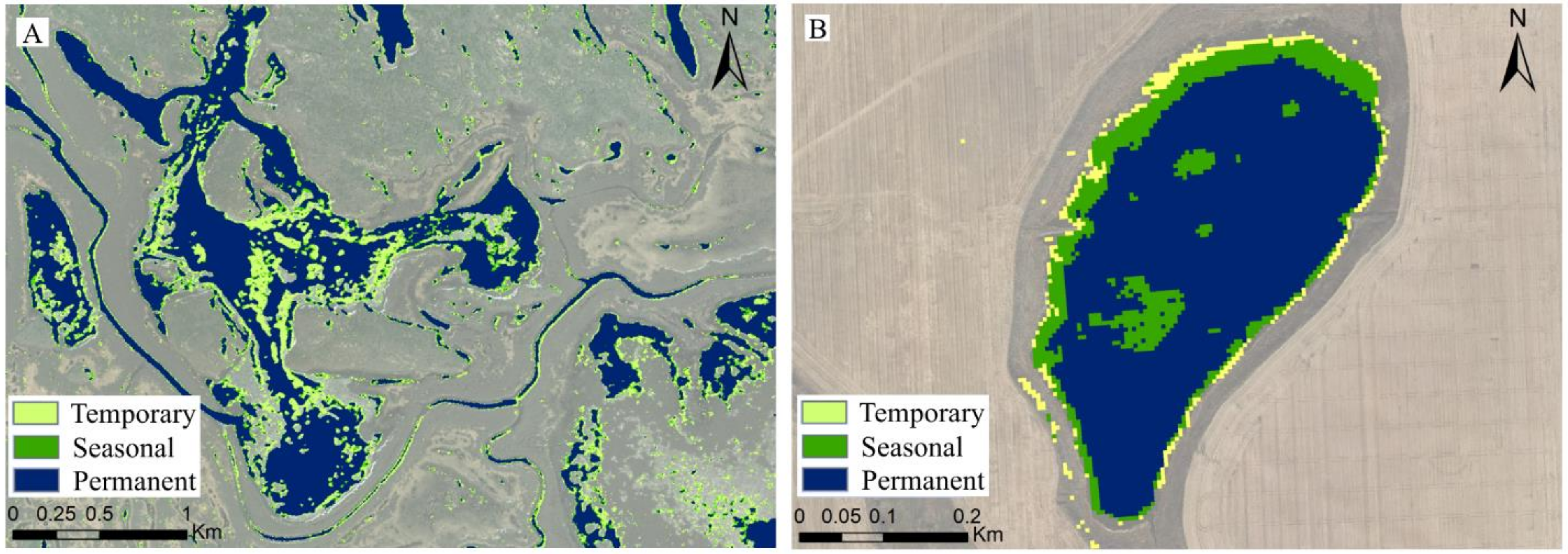
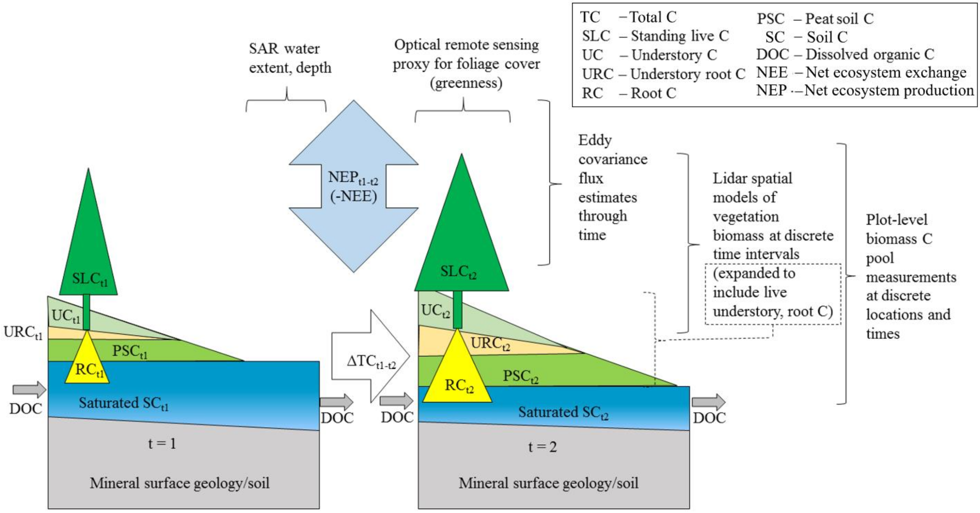
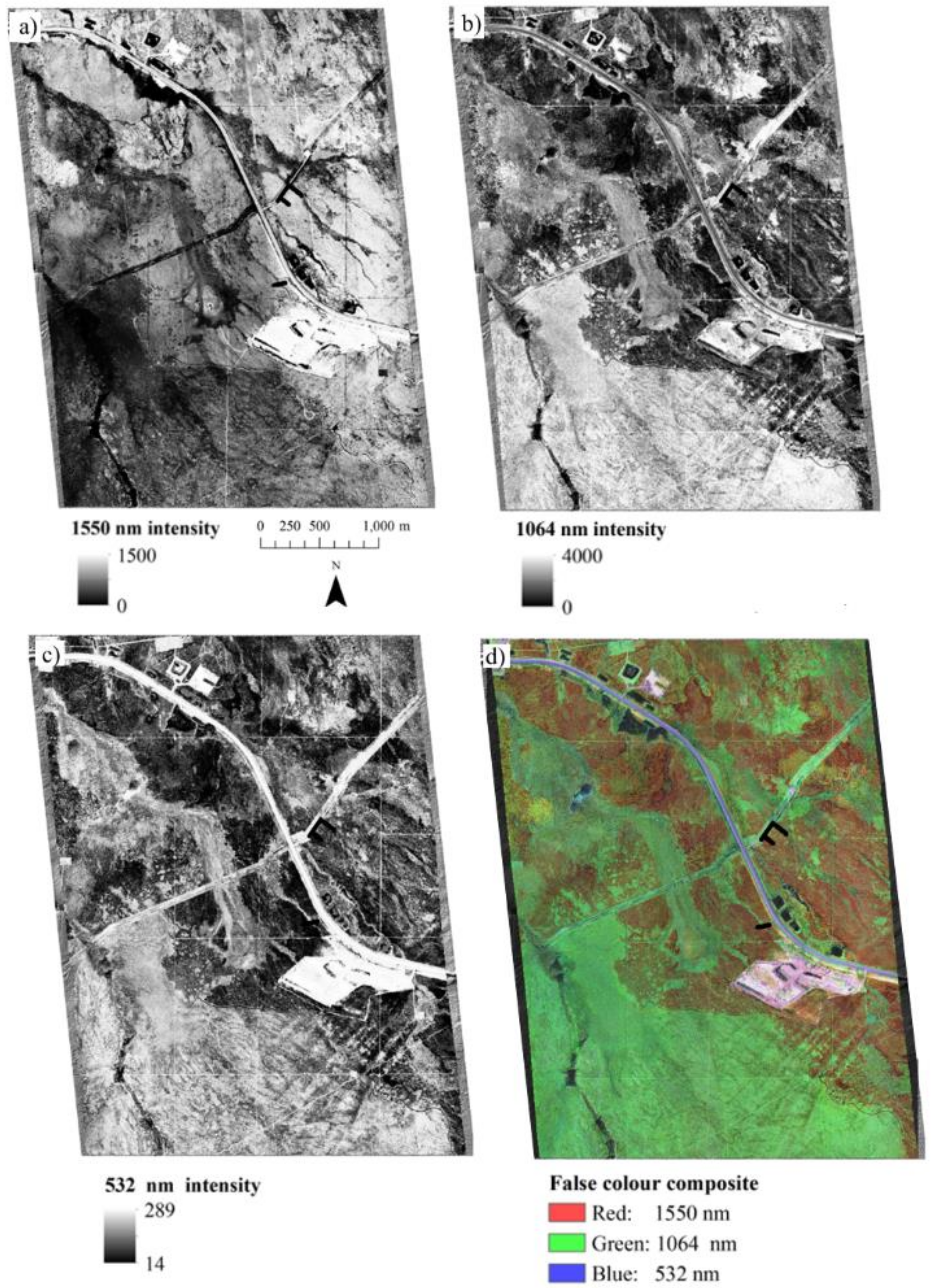
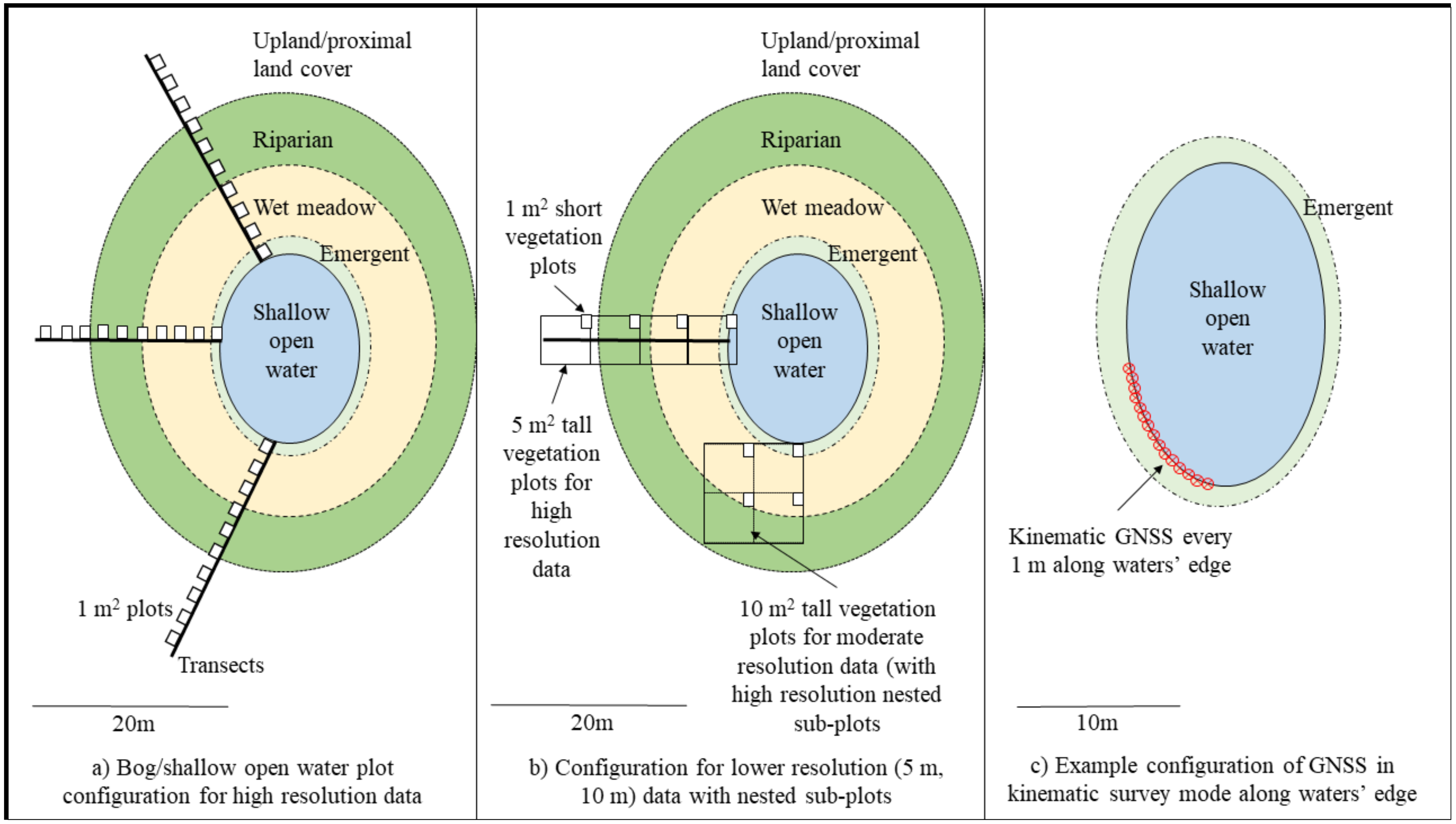
Figure 1. (a) Optical Worldview-2 panchromatic band (0.3 m pixel resolution) for a bog/shallow open water wetland in central Alberta, Canada. Identifiable shrubs along the transition zone between the wetland and riparian zone are visually observed in the images; (b) visible colour composite from Worldview-2 for the same bog. Pixel resolution is 1.4 m, smaller shrubs are within pixels and are averaged, making the boundary between shrubs and riparian area easier to discern; (c) Sentinel-2 data (visible colour composite) where transition zone is integrated with riparian and forest and wetland edge can be identified. Red outlines represent object-oriented segmentation associated with spectral reflectance differences of vegetation and soil moisture, riparian and forested zones.
Remotesensing 12 01321 g001
Figure 2. Multi-polarization data from Radarsat-2 illustrating mixtures of coherence statistics. These statistics are associated with mean coherence (mostly red upland vegetation), standard deviation coherence (mixture of mostly green and some red with variation depending on vegetation structure) and blue to blue-green related to open water, aquatic and flooded vegetation within the Peace Athabasca Delta, Alberta Canada.
Remotesensing 12 01321 g002
Figure 3. (A) Synthetic aperture radar (SAR)-derived hydroperiod (2015) in the Peace-Athabasca Delta, Alberta; (B) RapidEye-derived hydroperiod (2015) illustrating optically-based water extent variations in an agricultural environment east of Calgary, Alberta. Both images have a spatial resolution of 5 m and include a series of six images acquired during the growing season (April to September).
Remotesensing 12 01321 g003
Figure 4. Schematic of carbon pool changes over time with succession/lowering water table and remote sensing measurements for boreal peatlands. Adapted from [347] (for forested environments).
Remotesensing 12 01321 g004
Figure 5. Gridded laser return intensities for burned and unburned boreal forest/peatland environment, where (a) is 1550 nm (channel 1), (b) is 1064 nm (channel 2), (c) is 532 nm (channel 3) and (d) is a false colour composite of the intensity images within red, green and blue colour bands. Red represents the area burned by wildfire, whereas green represents healthy vegetation (mostly forest and some peatlands).
Remotesensing 12 01321 g005
Figure 6. Illustration of transect and plot set up example for (a) high resolution data (~1 m2), (b) moderate resolution data (10 m2) with understory plots and (c) kinematic survey along the waters’ edge required for validation of water extent.
Remotesensing 12 01321 g006
Table 1. Current (and future) remote sensing technologies used for mapping wetlands, ranked from high to low spectral resolution per class from 178 peer reviewed journal articles. Pan = panchromatic band.
TypeSensorSpatial Resolution (m)Number of BandsYears of OperationRevisit Time (Days)References
Airborne photographyBlack/white camera0.05–51OngoingOn demand[37,38,39,40,41,42,43,44,45,46,47,48,49,50]
Near infrared camera0.05–51OngoingOn demand[51,52,53,54]
Multi-spectral camera0.05–5VariesOngoingOn demand[38,40,52,53,54,55,56,57]
Airborne
Hyper-spectral
PROBE-1Varies1281998-On demand[58]
MIVISVaries102Early 1990sOn demand[59,60,61]
ROSISVaries1151992-On demand[59]
Hymap3.5–101281998On demand[62,63,64,65,66]
SASI0.25–15160UnknownOn demand[67,68]
CASI0.25–152881989-On demand[59,67,68,69,70,71,72]
AVIRIS172241987-On demand[73,74,75,76,77,78,79,80]
Satellite hyper-spectralHyperion302422000–2017On demand[22,81,82,83]
Satellite multi-spectralWorldView series~1.4 (0.3 pan)82007-1–2[80,82,84,85,86,87,88,89]
GeoSat1.84 (0.46 pan)4 (+ pan)1985–1990On demand[90]
Pleiades 1A, 1B2 (0.5 pan)4 (+ pan)2011-1[26]
Quickbird3 (0.65 pan)4 (+ pan)2001–20141–3.5[54,57,59,88,91,92,93,94,95]
Planet CubeSat, Dove, etc.432013-1[96]
IKONOS4 (1 pan)4 (+ pan)2000–20153[21,27,48,59,97,98,99,100,101,102,103,104,105,106,107]
KOMPSAT series4–5 (0.55–1 pan)4 (+ pan)1999-On demand[57]
RapidEye552009-5.5[80,87,96,108,109,110,111]
SPOT series5, 10, 20 (2.5 pan)4 (+ pan)1986-5[44,57,112,113,114,115]
ASTER15–90141999-16[22]
Sentinel-2A, B10, 20, 60122015-5[26,68,86,116]
Landsat TM3071982–201216[22,46,47,56,68,108,117,118,119,120,121,122,123,124,125]
Landsat ETM+30 (15 pan)81999-16[46,79,80,82,120,126,127]
Landsat OLI30 (15 pan)92013-16[68,86,127,128,129]
Landsat MSS6051972–199916[45,117]
MODIS250, 500, 1000361999-1 – 2[23,130,131,132,133,134,135,136,137]
AVHRR series110061978-1[45,118,130,138,139]
MERIS300, 1200152002–20123[140,141,142,143,144,145,146]
Synthetic aperture radarTerraSAR-X1, 3, 161: X-band2008-11[147,148]
NISAR3–102: L-band, S-band2020 (planned)12[149]
Radarsat Constellation Mission3–1003 satellites: C-band201912[150]
Sentinel-1A, B3.5–401: C-band2014-12[116,151]
RADARSAT-28–1001: C-band2007-24[25,30,111,128,152,153,154,155]
JERS-1181: L-band1992–199844[156,157,158]
ENVISAT ASAR30, 150, 10001: C-band2002–201235[159,160,161,162]
RADARSAT-18–1001: C-band1999–201324[119,163,164]
ALOS PALSAR10, 1001: L-band2006–200814[155,165,166,167,168]
ERS-1, -2251: C-band1991–2011On demand[169,170]
SeaSAT251: L-band1978Unknown[171,172]
SMAP1000–30001: L-band2015-2 – 3[173,174]
Shuttle Imaging Radar (SIR)253: C-band, X-band, L-band1981, 1984, 1994Single acquisitions[165,175,176]
Geosat Follow-OnNot available1: ku-band1998–200817[177]
Jason series36,0001: S-band2001-10[177,178,179]
Airborne lidarBathymetric lidarVaries based on spot spacing; 0.5–52Varies: mid-2000sOn demand[85]
Discrete return lidarVaries based on spot spacing; 0.5–511998–(commercial systems)On demand[19,20,28,29,30,50,84,124,137,180,181,182,183,184,185,186,187,188,189,190]
Multi-spectral lidarVaries based on spot spacing; 0.5–532014-On demand[191,192,193,194]
Table 2. Average and standard deviation of data product accuracy compared with measurements collected in the field and accurately located using Global Navigation Satellite System (GNSS) from combined remotely sensed data based on pixel resolution. Bold numbers illustrate pixel resolution range of highest average accuracy; n = the number of comparison results from the literature (205 examples in total); and NA represents applications where remotely sensed data products are not available for wetlands at that pixel resolution.
Ramsar Process GroupingApplicationAverage (stdev.) Accuracy (%) of Remotely Sensed Data Products from Wetlands
High (≤10 m)Medium (11 to 30 m)Low (≥30 m)
Wetland Classification and ExtentLand cover classification (wetland/no wetland)85 (12) (n = 8)76 (21) (n = 10)45 (32) (n = 8)
Wetland class84 (8) (n = 22)79 (14) (n = 13)71 (13) (n = 7)
Wetland form/type80 (8) (n = 3)55 (6) (n = 2)NA
Hydrological Regime and Water cyclingWater extent87 (11) (n = 11)86 (17) (n = 18)76 (4) (n = 2)
Soil moistureNA61 (8) (n = 2)69 (15) (n = 3)
Topography78 (8) (n = 10)NANA
Biogeochemical ProcessesWater chemistry81 (7) (n = 3)78 (12) (n = 12)81 (10) (n = 4)
Mine spill detectionNA89 (9) (n = 3)NA
Carbon Uptake and Biological productivitySpecies identification81 (19) (n = 27)78 (11) (n = 5)NA
Ecosystem productivity71 (16) (n = 5)59 (20) (n = 5)43 (9) (n = 5)
Foliage biochemistry59 (13) (n = 2)NA57 (39) (n = 3)
Vegetation structure78 (2) (n = 4)71 (NA) (n = 2)NA
Habitats84 (13) (n = 3)19 (9) (n = 3)NA

